This note is the reader companion to the interactive deck. It follows the deck's order. Every number below is printed by workbook.ipynb in this folder and is stored in numbers.json; a widget at its default state shows the same value. The lecture stands alone: it introduces each scenario on its own terms.
The setting is two programs joined by one file. The engine (a crowd-dynamics library, JuPedSim) moves simulated walkers and writes where each walker was at every frame. The measurer (an analysis library, PedPy) reads that file and turns positions into density and speed. They never share memory. They agree on the layout of one file, like two technicians who never meet and share only a standard form. Either technician can be replaced if the form stays the same. The first five sections build and break the model that writes the file; sections 6 to 9 follow the file into the measurer; section 10 asks what a random seed can and cannot vary.
All runs in the workbook use one ring: a periodic single-file corridor of length L = 17.3 m. Defaults are desired speed v0 = 1.2 m/s, time gap T = 1.0 s, body length l = 0.3 m, N = 20 walkers, time step dt = 0.05 s, seed 1. The starting positions are evenly spaced slots displaced by a uniform random amount of up to 10 % of the spacing. That 10 % is an assumption of this course, not a value from the literature.
1. Space per person sets the pace (the speed law)
Deck widget: SpeedLaw.
A first-order speed model gives each walker a speed from the free distance in front of her, not a force. The collision-free speed model uses a piecewise-linear optimal-velocity function (tordeux2016_5e66 ↗):
Here s is the gap between centres, l the pedestrian diameter, v0 the desired speed and T the time gap. The published parameter set is v0 = 1.2 m/s, l = 0.3 m, T = 1 s. The function is zero until the gap exceeds one body length, rises with slope 1/T, and is capped at v0. Because V(s) = 0 for every s ≤ l and V is never negative, a walker cannot be driven into the one in front: the model is collision-free by construction.
Rearranged on the sloping part, s = l + T v. The space a walker needs grows linearly with her speed. This is the form of the empirical required-length law d = a + b v (seyfried2006_f4db ↗, which finds a = 0.36 m and b = 0.56 s in good agreement with single-file data for a different, second-order model). The numbers are not interchangeable between models; the shape is the same.
Equilibrium on a ring. Put N walkers on a ring of length L at uniform spacing s = L/N. Then every walker sees the same gap and moves at V(L/N). With linear density ρ = 1/s (ped/m) the flow is J(ρ) = ρ V(1/ρ). Two branches follow:
In words: a walker needs one body plus T seconds of travel in front of her; with less than that she slows in proportion, and the congested branch of the flow is a straight line whose slope is minus body length over time gap.
Worked numbers at the defaults (workbook section 1). The probe spacing is L/N = 0.865 m, so V = (0.865 - 0.3)/1.0 = 0.565 m/s and J = 0.653 ped/s. The critical density is 0.667 ped/m, capacity 0.800 ped/s, jam density 3.33 ped/m, wave speed -0.30 m/s. A brute-force scan of J(ρ) returns the same capacity (0.800 ped/s at 0.667 ped/m) and a congested-branch slope of -0.3. The free-flow branch ends at a spacing of l + v0 T = 1.5 m.
With the parameter set of xu2019_05d4 ↗ for single file (v0 = 1.34 m/s, T = 1.06 s, l = 2a = 0.36 m from a circle radius a = 0.18 m) the same formulas give 0.476 m/s at the probe, ρ_c = 0.562 ped/m, J_max = 0.753 ped/s, ρ_jam = 2.78 ped/m and wave speed -0.34 m/s. In single file only the speed sub-model matters, because nobody can overtake; that paper reports the direction and shape sub-models as insignificant there.
A measured reference exists: the single-file fit v(w) = U(1 - exp(-(w - w_m)/w_s)) with U = 1.26 m/s, w_m = 0.31 m, w_s = 0.93 m, where w is the distance to the next person (maury2018_d24a ↗, section 9.4, fitted to two single-file data sets). Its flow peaks at 0.66 ped/s near 1.02 ped/m. At the probe spacing it gives 0.566 m/s.
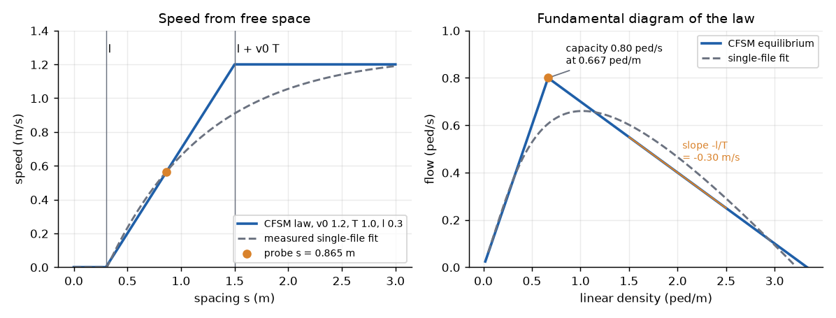
Break it. Set T = 0.3 s and l = 0.2 m. Capacity becomes v0/(l + v0 T) = 2.143 ped/s, 3.25 times the capacity of the measured fit. A parameter set can make the model carry far more than any single-file measurement; the law does not object.
Concept check. Why does capacity fall when the body length grows, although a bigger body does not slow a walker in free flow? Answer: capacity is v0/(l + v0 T). A walker at speed v0 needs l + v0 T of ring, so a larger l raises that space and fewer walkers pass a point per second, even though no single walker is slower in free flow.
2. A ring of walkers (the engine running)
Deck widget: CorridorCSM.
Integrate the model on the ring with explicit Euler and a parallel update, so that every walker uses the gaps of the previous step:
Walker N-1 follows walker 0 shifted by L. The corridor length 17.3 m is the periodic length that seyfried2006_f4db ↗ chose to compare with the empirical single-file experiment; the same paper reports no notable finite-size effect between 17.3, 20 and 50 m.
In words: each walker looks only at the gap ahead, and the ring settles because every gap is pulled toward its neighbour's gap.
Why the mean speed cannot show relaxation. The gaps sum to L at every step, since the ring closes. While every gap lies between l and l + v0 T, V is linear, so the mean speed is (mean gap - l)/T = (L/N - l)/T exactly, whatever the arrangement. The workbook confirms it: from the jittered start the mean speed equals 0.565 m/s at step 0, and its largest deviation from 0.565 over 120 s is below 1e-12. The spread of the gaps is what relaxes.
Worked numbers (seed 1). The start has gaps from 0.746 to 0.963 m (sd 0.0664 m). The sd of the gaps is 0.0051 m at 10 s, 0.0020 m at 30 s and 0.00049 m at 60 s. At t = 60 s the mean speed is 0.565 m/s (equilibrium 0.565), the minimum gap 0.864 m and there are no overlaps; the highlighted walker 0 has gap 0.866 m and speed 0.566 m/s. The slowest gap mode decays with time constant T/(1 - cos(2π/N)) = 20.4 s. This follows from the small-gap dynamics dg_i/dt = (g_{i+1} - g_i)/T, whose Fourier mode k decays at rate (1 - cos(2πk/N))/T; maury2018_d24a ↗ (section 2.1, Remark 2.4) gives the same relaxation rate, φ'(w_eq)(1 - cos(2π/N)), for a general follow-the-leader law on a periodic corridor, where φ' = 1/T here.
Jammed start. Place the walkers back to back, x_i = i l. All 19 walkers except the front one have gap l and speed 0. The block is 6.0 m long, and the front walker faces a free gap of 11.6 m. The mean speed starts at 0.06 m/s. The start of motion travels down the block one walker per step but with a vanishing amplitude: every walker has a non-zero speed (above 1e-9 m/s) from 3.5 s, and the last walker in the block moves faster than 1 mm/s from 8.5 s. From 8.5 s no walker is capped at v0 any more, and the mean speed stays within 2 % of 0.565 m/s from 8.25 s. The jam dissolves from its front backward, as the right panel shows.
Infeasible geometry. N bodies of length l need N l ≤ L. With N = 60 and l = 0.3 m, N l = 18.0 m exceeds 17.3 m, so the ring cannot be filled. The largest feasible N at l = 0.3 m is 57.
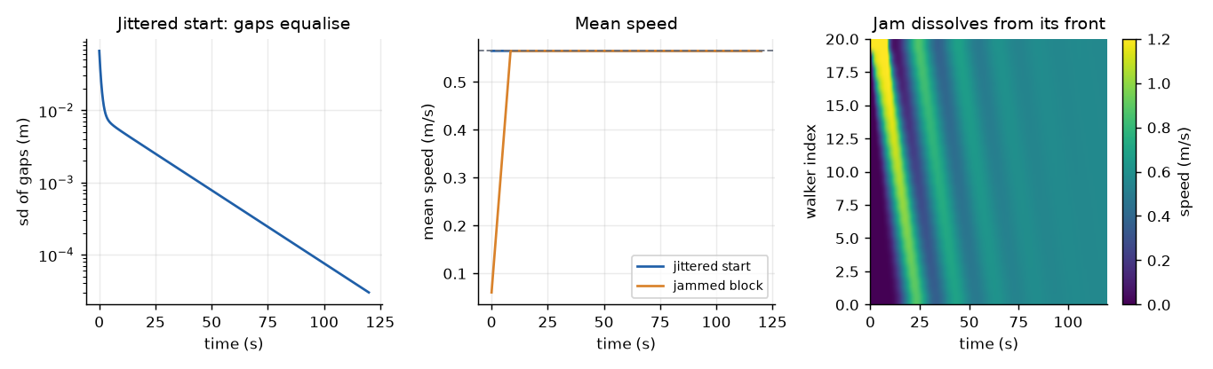
Concept check. The mean speed is exactly the equilibrium value at t = 0. Does that mean the ring is at equilibrium? Answer: no. The mean depends only on the sum of gaps; equilibrium also needs equal gaps, and the sd of the gaps is still 0.0664 m at t = 0.
3. Simulated points against the measured curve (the fundamental diagram)
Deck widget: FundamentalDiagram.
Sweep N, record the steady mean speed of each run and plot speed against density. Each run lasts 120 s and the mean is taken over the last 60 s. Two references are used, and their densities are in different units.
- The measured single-file fit above, on linear density ρ = N/L in ped/m.
- The Weidmann floor-density curve, as quoted in maury2018_d24a ↗: u = 1.34 (1 - exp(-1.913 (1/ρ - 1/5.4))), ρ in ped/m², maximum density 5.4 ped/m².
A ring of single-file walkers measures ped/m. Putting it on the Weidmann axis needs a lane width w with ρ = ρ_1/w. The corpus gives no single-file lane width, so w is an assumption.
Simulated points (Tordeux parameter set) against the fit:
| N | ρ (ped/m) | simulated (m/s) | single-file fit (m/s) |
|---|---|---|---|
| 2 | 0.116 | 1.200 | 1.260 |
| 4 | 0.231 | 1.200 | 1.243 |
| 8 | 0.462 | 1.200 | 1.088 |
| 12 | 0.694 | 1.142 | 0.887 |
| 16 | 0.925 | 0.781 | 0.710 |
| 20 | 1.156 | 0.565 | 0.566 |
| 24 | 1.387 | 0.421 | 0.450 |
| 30 | 1.734 | 0.277 | 0.314 |
| 36 | 2.081 | 0.181 | 0.211 |
| 42 | 2.428 | 0.112 | 0.131 |
| 48 | 2.775 | 0.060 | 0.066 |
| 54 | 3.121 | 0.020 | 0.014 |
| 60 | 3.468 | cannot place 60 bodies of 0.3 m on 17.3 m | 0 |
At every feasible N the simulated mean equals the equilibrium V(L/N) to three decimals, as section 2 predicts for a jittered start. The sweep therefore checks the integrator; the information is in the comparison with the fit.
Misfit against the fit, RMSE over 0.5 to 2.5 ped/m: the equilibrium curve of the Tordeux set is 0.093 m/s from the fit, and its seven simulated points in that range are 0.102 m/s. For the Xu set the values are 0.121 and 0.098 m/s. At N = 20 the two agree (0.565 and 0.566 m/s); at N = 12 they differ by 0.255 m/s. This week reports the misfit for two published parameter sets. It does not fit them.
Free speed is not one number. Values reported across sources run from 1.2 m/s (the model's default) through 1.24 (Seyfried, normal with sd 0.05) and 1.30 with sd 0.21 (as quoted by Maury) to 1.34 (Weidmann) and 1.55 with sd 0.18 in zhang2012_ab8c ↗. The choice of v0 moves the whole free-flow branch.
Break it: the unit assumption. At N = 20 the linear density is 1.156 ped/m. With w = 0.8 m the floor density is 1.445 ped/m² and the Weidmann curve gives 0.832 m/s. With w = 1.0 m it is 1.156 ped/m² and the curve gives 0.975 m/s, against 0.565 m/s from the model. Over 0.5 to 2.5 ped/m the RMSE between the model's equilibrium curve and the Weidmann curve is 0.231 m/s at w = 0.8 m and 0.368 m/s at w = 1.0 m. Scanning w from 0.40 to 1.20 m, the smallest RMSE is 0.072 m/s at w = 0.57 m. So the agreement between a single-file model and a two-dimensional curve is set by a number nobody measured. When the digits of ped/m and ped/m² coincide, the eye reads agreement; the RMSE reads the assumption.
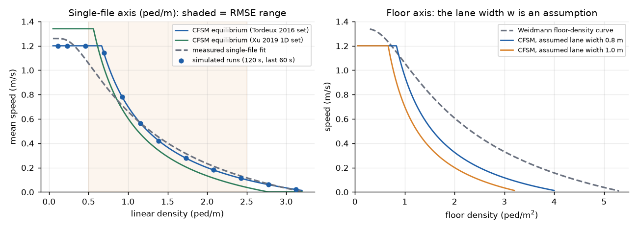
Concept check. Across the feasible points (12 for the Tordeux set, 11 for the Xu set) the Spearman rank correlation between density and speed is -0.99 for both parameter sets, although their RMSE values differ (0.093 and 0.121 m/s). What does the correlation say? Answer: order only. It is not -1.00 because the free-flow plateau (N = 2, 4, 8, all 1.200 m/s) produces ties. A rank correlation says that speed falls as density rises; it does not say by how much, and it cannot separate two parameter sets.
4. Break it: a time step too large for the time gap
Deck widget: EulerStep.
The corpus states no step bound for this model. The bound below is derived here.
One walker behind a stopped leader. One Euler step gives a new gap s' = s - dt V(s) = s - dt (s - l)/T, so
which falls below l, an overlap, exactly when dt > T. Numerically, starting at s = 0.5 m with l = 0.3 m and T = 1 s, the next gap is 0.40 m for dt = 0.5 s, 0.30 m for dt = 1.0 s, 0.28 m for dt = 1.1 s, 0.20 m for dt = 1.5 s and 0.10 m for dt = 2.0 s.
A ring on the congested branch. With λ = dt/T the gap update is g_i' = (1 - λ) g_i + λ g_{i+1}. The alternating mode, g_{i+1} = -g_i, is multiplied by 1 - 2λ per step:
For dt < T this is below 1 and differences decay; for dt > T it is above 1 and small differences between neighbours grow. The workbook measures the factor on a pure alternating start: 0.90 at dt = 0.05 s, 0.00 at dt = 0.5 s and -2.00 at dt = 1.5 s, as the formula says.
In words: a step longer than the time gap lets a walker cover more than the free space in front before she looks again.
The continuous model cannot produce stop-and-go waves. tordeux2016_5e66 ↗ states that the model is intrinsically collision-free with no overlapping at any density, and its conclusion lists stop-and-go among the phenomena the model does not describe. Anything that looks like stop-and-go in the space-time picture below is therefore the integrator, not pedestrians.
Ring results, 60 s from the seed-1 jittered start:
| dt (s) | λ | |g_π| | overlap onsets per minute | min gap / l at end | walker-steps at zero speed |
|---|---|---|---|---|---|
| 0.005 | 0.005 | 0.99 | 0 | 2.88 | 0 |
| 0.05 (default) | 0.05 | 0.90 | 0 | 2.88 | 0 |
| 0.9 | 0.9 | 0.80 | 0 | 2.85 | 0 |
| 1.0 | 1.0 | 1.00 | 0 | 2.49 | 0 |
| 1.1 | 1.1 | 1.20 | 326 | 0.67 | 32.5 % |
| 1.5 | 1.5 | 2.00 | 285 | -0.92 | 43.1 % |
An overlap onset is a walker whose gap drops below l after having been at least l in the previous step. A negative minimum gap means one walker has passed through another. The lowest gap over the default run is 2.49 l (the start); at the end it is 2.88 l.
Published step sizes are 0.01 s in the collision-free speed model paper, 0.05 s in xu2019_05d4 ↗ and 0.001 s for a second-order hard-body model in seyfried2006_f4db ↗. The containerised engine used in this course defaults to a time step of 0.05 s (see the provenance appendix).
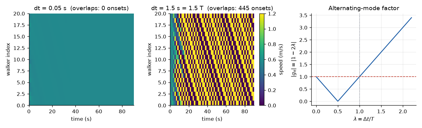
Concept check. At dt = T exactly, |g_π| = 1 and the stopped-leader gap lands on l. Why is that not yet an overlap in the run (table row dt = 1.0)? Answer: the overlap condition is strict, s' < l; at λ = 1 the update maps to l with no undershoot, and the alternating mode neither grows nor decays.
5. Break it: a body too small (or too large) for the geometry
Deck widget: BodySize.
Body length sets the jam density 1/l and, with v0 T, the critical density 1/(l + v0 T). The number of bodies that can be placed on the ring is at most
which is 57 at l = 0.3 m. Table of the workbook: l = 0.1, 0.2, 0.3, 0.4, 0.6 m gives N_max = 173, 86, 57, 43, 28 and jam density 10, 5, 3.33, 2.5, 1.67 ped/m. With v0 T = 1.2 m the critical density and capacity are 0.714 ped/m and 0.857 ped/s at l = 0.2 m, 0.667 ped/m and 0.800 ped/s at l = 0.3 m, and 0.556 ped/m and 0.667 ped/s at l = 0.6 m.
In words: the model walks only as crowded as its bodies are big.
Too small. At a spacing of 1.4 m and l = 0.2 m the model gives 1.20 m/s (1.10 m/s with the default l = 0.3 m), while the single-file fit gives 0.87 m/s. At N = 60 and l = 0.2 m the spacing is 0.2883 m: the model walks at 0.088 m/s (equilibrium and simulation at 60 s agree, and the starting gaps are all above l). The measured fit puts speed at zero for any spacing below its minimum distance w_m = 0.31 m. The model with a small body therefore walks at spacings the measurement says nobody reaches. The measured w_m is a check on l.
The small body also moves the congested branch upward: at any density above ρ_c the flow is higher than for l = 0.3 m. The free-flow branch itself ends slightly later (0.714 against 0.667 ped/m); the larger effect is on the congested branch.
Too large. At l = 0.6 m the ring holds 28 bodies. N = 30 needs 18.0 m of body on 17.3 m of ring, so the run cannot start.
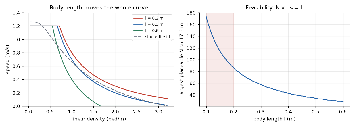
Concept check. A colleague sets l = 0.1 m to "fit more people in". Which two checks in this section catch it? Answer: the spacing at the target N falls below the measured minimum distance 0.31 m, and the jam density 1/l = 10 ped/m is above the largest linear density (about 3 ped/m) in the measured single-file data.
6. The file between the engine and the measurer (the trajectory contract)
Deck widget: TrajectoryContract.
The engine writes one file the measurer is required to read. It has five typed columns, one row per walker per frame:
| Column | Type | Meaning |
|---|---|---|
frame |
int32 | frame number 0, 1, 2, ... |
t_s |
float64 | clock time of the frame, seconds |
agent_id |
int32 | which walker this row is about |
x |
float64 | position, metres |
y |
float64 | position, metres |
The two programs are written by different people, depend on different libraries and run in separate sealed boxes. They share this file and nothing else. As long as the engine writes those columns and the measurer reads them, neither needs to know about the other.
The row count is predictable: rows = N × duration/dt. For N = 20, 180 s and dt = 0.05 s this is 3600 frames and 72,000 rows; the workbook builds exactly that from the ring, mapping arc position onto a circle of circumference 17.3 m (radius 2.7534 m).
A consumer must refuse a file that breaks the contract rather than return a plausible number. The validator in the workbook checks, in order: column names and order, dtypes, row count against the prediction, uniqueness of (frame, agent_id) keys and a plausibility gate. The gate computes the largest speed between consecutive frames of one walker and refuses the file above a ceiling; the ceiling of 3 m/s is an assumption. A type check is necessary and not sufficient.
Verdicts on the clean file and on five corruptions:
| File | Failed checks |
|---|---|
| clean | none (largest speed 0.663 m/s) |
t_s renamed to time |
names, dtypes |
x stored as float32 |
dtypes |
agent_id dropped |
names, dtypes |
x, y written in centimetres |
plausibility only (largest speed 66.34 m/s) |
| one frame written twice | row count (72,020 against 72,000), unique keys (20 duplicates) |
The centimetre file passes every schema check and returns speeds one hundred times too large. The largest clean speed, 0.663 m/s, is the fastest walker of the jittered start; it is not the desired speed 1.2 m/s.
The measurer's own output has the shape of a per-window summary. Its columns are t_s (float64), mean_density_ped_m2 (float64), mean_speed_m_s (float64) and n_active (int32). Toy rows computed by the workbook for the 2 m section at 1 s windows starting at 60, 61 and 62 s are density 1.446 ped/m² (the linear Voronoi density 1.156 ped/m divided by an assumed lane width of 0.8 m), speed 0.564 m/s and n_active 2.
In words: the file is the only thing the two programs agree on, so the check at the file is where errors are caught or lost. Week 4 treats units and clocks between stages in depth; this week only names the gate.
Concept check. Why does a duplicated frame need its own test? Answer: every dtype is right and every value is plausible, but the row count and the key set are wrong; and a finite difference across the duplicated pair returns zero speed followed by a jump (section 8).
7. Measuring density: count in a section, or Voronoi cell
Deck widget: MeasureSection.
The measurer sees positions, not the model. The classic density counts walkers inside a measurement section and divides by its size. When the section is comparable to a body it jumps as walkers enter and leave, with fluctuations of the same order as the density itself (liddle2022_ee2c ↗). The Voronoi method gives each walker the floor closer to her than to anyone else, and integrates one over the cell size across the section. That paper reports much smaller fluctuations; zhang2012_ab8c ↗ chose it for small scatter and high resolution and used a 2 m measurement section.
In one dimension the cell is exact: half the distance to each neighbour,
In words: counting heads in a small box is noisy; sharing the floor out by nearest person is not.
Worked numbers: ring of 20 at equilibrium, section starting at 7.65 m, samples at every frame from 60 s to 120 s. The true density N/L is 1.156 ped/m.
| section L_m | classic mean, sd (ped/m) | values seen | Voronoi mean, sd (ped/m) |
|---|---|---|---|
| 2.0 m | 1.155, 0.231 | 1.00 and 1.50 | 1.156, 0.0003 |
| 0.5 m | 1.162, 0.987 | 0 and 2.00 | 1.156, 0.0003 |
| 0.3 m | 1.153, 1.585 | 0 and 3.33 | 1.156, 0.0003 |
The classic sd exceeds its own mean for section lengths of 0.4 m and below (scan from 0.2 m in steps of 0.05 m); at 0.5 m the ratio is 0.85, and near one spacing (0.85 m) it is 0.13. The Voronoi sd is tiny here because the relaxed ring is almost perfectly regular; on a real file with irregular spacing it will be larger. The section position does not matter on a uniform ring (Voronoi mean 1.156 at 2.0 m and 12.0 m).
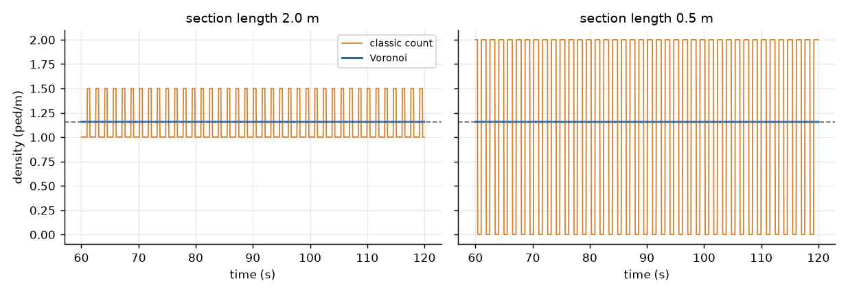
Concept check. A section is 0.3 m long and the classic density at one frame is 3.33 ped/m. Is the crowd dense? Answer: not necessarily. One walker is inside a box of 0.3 m, or none is; the true density is 1.156 ped/m.
8. Measuring speed: finite differences and the periodic seam
Deck widget: SpeedEstimator.
Speed is not stored in the trajectory file; the measurer differences positions:
liddle2022_ee2c ↗ uses a window of 0.2 s, 5 frames at 25 frames per second. Here k = 4 frames at dt = 0.05 s gives the same 0.2 s. For odd k the workbook uses x(n + ceil(k/2)) - x(n - floor(k/2)).
Noise. If the stored position carries independent noise of sd σ_x, the speed error has sd √2 σ_x/(k dt). At σ_x = 0.02 m this is 0.566 m/s for k = 1, 0.141 m/s for k = 4 and 0.028 m/s for k = 20; measured on seeded noise the workbook finds 0.566, 0.138 and 0.028. At k = 1 the noise is as large as the walking speed. The workbook cannot show the opposite cost of a long window, blur of real speed changes, because a relaxed ring has constant speed.
The seam. The file stores the wrapped coordinate, so a walker crossing the seam jumps from x near L to x near 0. An unwrapped difference returns v - L/(k dt). For L = 17.3 m and k dt = 0.2 s, L/(k dt) = 86.5 m/s, so a walker at 0.565 m/s gives -85.94 m/s (the workbook's sample for walker 0 is -85.93 m/s). Walker 0 crosses twice in the 60 s window, each crossing affecting the 4 samples whose window straddles it, so 8 samples in all. The mean speed over the window is 0.565 m/s with the difference unwrapped to the nearest image (d - L round(d/L)) and -0.012 m/s without. The mean absolute error against the model speed is below 1e-5 m/s unwrapped and 0.577 m/s not.
In words: speed is a difference of two positions, so any jump in position is a speed. The same happens when frames are dropped or duplicated, which is why the contract check in section 6 includes a duplicate-frame test.
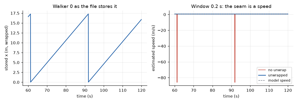
Concept check. Someone reports mean speed -0.012 m/s for walkers who are visibly walking. Which two lines of the contract check would you run first? Answer: the plausibility gate on maximum speed, and the seam test (any consecutive-frame jump larger than L/2 in a wrapped coordinate).
9. Warm-up is not data (steady state and discard)
Deck widget: TransientDiscard.
A run starts from an artificial arrangement, and averages must be taken over the stationary part only. zhang2012_ab8c ↗ selected stationary periods by inspecting the density and speed series and kept one frame per second before building the fundamental diagram. The discard fraction is a choice to be declared in the run's configuration, not a constant of nature.
Worked numbers with the jammed start, N = 20, run 120 s, f = 0.3 (t_d = 36 s). The mean speed with the discard is 0.565 m/s, without it 0.547 m/s, a bias of -0.018 m/s. The mean speed stays within 2 % of its final value from 8.25 s (7.5 s at a 10 % tolerance, 8.35 s at 1 %). From a jittered start the bias is zero, because the mean speed never leaves 0.565 m/s.
Break it. Take a 30 s run with no discard: the mean is 0.494 m/s, 0.071 m/s below the equilibrium 0.565 (12.6 %). The point would sit off the curve of section 3 for a reason that has nothing to do with the model's parameters. A 30 % discard on the same run (9 s) recovers 0.565 m/s.
What stationary means. The mean speed is flat from 8 s, yet the gaps are still relaxing: their sd falls below 1 % of the mean gap only at 93.3 s. Section 2 explains it: once no walker is capped by v0 the mean speed depends only on the sum of the gaps. A stationarity test on the mean speed alone is therefore weak on this ring. A rough kinematic estimate, block length over wave speed, 6.0 m / 0.3 m/s = 20 s, does not match any of the three times measured (8.5 s for the last walker to move, 8.25 s for the mean, 93.3 s for the gaps); we did not test why. The lesson stands: declare the discard, and test stationarity on more than one quantity.
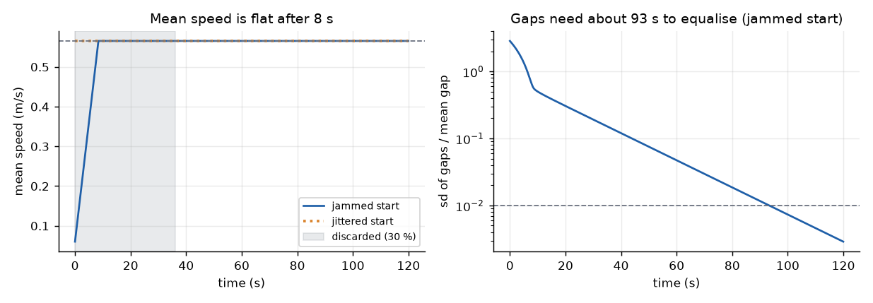
Concept check. Why does the jittered start need no discard for the mean speed, and is that a reason to skip the discard? Answer: its mean speed is exact from step 0 because no walker is capped; the discard is still declared because the configuration has not relaxed and other observables, such as the gap distribution, depend on it.
10. What a seed varies: repetition, heterogeneity and platoons
Deck widget: SeedsAndPlatoons.
With identical walkers and dt below T the equilibrium of section 2 is unique and stable, so every seed converges to the same mean speed V(L/N). Seeds that only move the start are repetitions of one steady state, not independent draws of a population. The containerised engine behind this chain takes no seed of its own; its wrapper seeds only the placement jitter of the spawn positions (curated note, see the appendix), so a run there is a repetition in this sense.
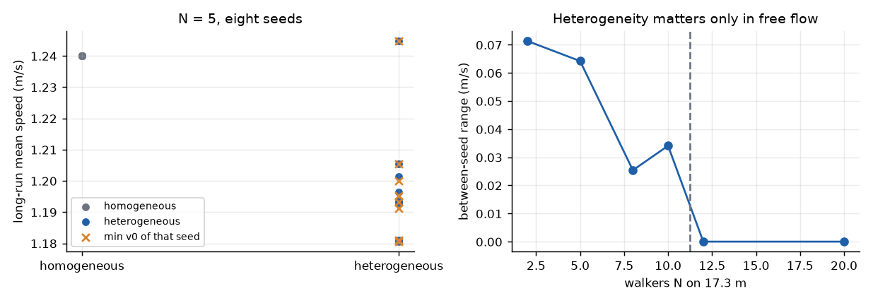
Workbook, N = 5, v0 = 1.24 m/s, eight seeds, 600 s, mean over the last 60 s: every seed gives 1.240 m/s, range 0.000; twenty seeds give an interval of half-width 0.000000. The evidence is one configuration, however many seeds you run. At N = 20 the eight seeds differ only in how long the gaps take to fall below 1 % of the mean gap (1.8 to 4.4 s); the long-run mean is 0.565 m/s for all of them.
Heterogeneity changes that. Draw each walker's desired speed from a normal distribution with mean 1.24 m/s and sd 0.05 m/s, the distribution used for single file in seyfried2006_f4db ↗. The draws here use Box-Muller on a second mulberry32 stream (seed + 100000). At low density nobody can overtake, so on a ring every walker ends up queued behind the slowest one, and the long-run mean tends to the minimum drawn v0:
The corpus is silent on this platoon result; it is derived here from the no-overtaking rule. Numbers for seed 1: the five desired speeds are 1.202, 1.200, 1.267, 1.249 and 1.208 m/s; the minimum is 1.200 and the long-run mean is 1.201 m/s. At 600 s two platoons remain, because the two slowest walkers (1.200 and 1.202) close at 0.002 m/s. Across the eight seeds the long-run means average 1.199 m/s, range 0.064 m/s, sd 0.020 m/s, with a 95 % half-width of 0.017 m/s (t distribution, n = 8); the largest gap between a seed's long-run mean and its minimum v0 is 0.0015 m/s. Four of the eight seeds have reached a single platoon.
Heterogeneity matters only where some walker is capped by her own v0. The between-seed range of the long-run mean by N (eight seeds, heterogeneous) is 0.0714 (N = 2), 0.0642 (5), 0.0254 (8), 0.0341 (10), then 0 at N = 12 and 20. With v0 = 1.24 m/s the critical count is L/(l + v0 T) = 11.2 walkers.
In words: a seed that only reshuffles the start gives the same answer eight times; a seed that draws who the walkers are gives a spread you can report.
Concept check. Twenty homogeneous seeds give a 95 % interval of zero width. What is wrong with reporting it? Answer: the seeds were not independent samples of anything; only the start moved. The zero width measures the determinism of the model, not the precision of an estimate. Week 7 develops this as replication versus repetition.
Exam questions and model answers
1. Landmarks. For v0 = 1.34 m/s, T = 1.06 s and l = 0.36 m compute the critical density, capacity, jam density and congested-branch wave speed of the equilibrium fundamental diagram on a periodic corridor.
Model answer. ρ_c = 1/(l + v0 T) = 1/(0.36 + 1.4204) = 0.562 ped/m. J_max = v0 ρ_c = 0.753 ped/s. ρ_jam = 1/l = 2.78 ped/m. c = -l/T = -0.34 m/s. These come from J = ρ v0 on the free branch and J = (1 - ρ l)/T on the congested branch, which meet at ρ_c.
2. Relaxed or not. A colleague checks that a ring simulation has "reached steady state" by watching the mean speed. Give a start for which this test is passed at t = 0 although the ring has not relaxed, and name a better diagnostic.
Model answer. Any start with all gaps between l and l + v0 T, for instance the jittered start with gap sd 0.0664 m. The gaps sum to L, so the mean speed is (L/N - l)/T exactly. Watch the spread of the gaps (or the min and max gap): its sd was 0.0051 m at 10 s and 0.00049 m at 60 s.
3. Time step. State the condition on dt under which one Euler step of the collision-free speed model can put a walker inside the one in front of her, derive it, and say what a run at dt = 1.5 T looks like.
Model answer. With a stopped leader s' = l + (s - l)(1 - dt/T), below l iff dt > T (derived here; the corpus states no bound). On a ring the alternating gap mode is multiplied by 1 - 2 dt/T, magnitude above 1 for dt > T. At dt = 1.5 T the factor is -2; the workbook run shows 285 overlap onsets per minute, walkers passing through each other (minimum gap -0.92 l) and 43 % of walker-steps at zero speed. The continuous model does not produce stop-and-go, so that pattern is the integrator.
4. A green schema. A trajectory file passes the column, dtype and row-count checks and yields a mean speed of 66 m/s. Diagnose it and say which check would have caught it.
Model answer. Positions written in centimetres: every type is right and the values are 100 times too large. A plausibility gate on the largest frame-to-frame speed (ceiling assumed 3 m/s) refuses it; the workbook's corrupted file reads 66.34 m/s. Week 4 treats units between stages in depth.
5. Two density units. A single-file simulation is compared with the Weidmann curve. What must be assumed, and what does the comparison then measure?
Model answer. A single-file ring measures ped/m; the Weidmann curve is in ped/m². Converting needs a lane width w, ρ = ρ_1/w, and the corpus gives none for single file, so it is an assumption. The RMSE between the two curves depends on it: 0.231 m/s at w = 0.8 m, 0.368 m/s at w = 1.0 m, 0.072 m/s at w = 0.57 m. The comparison then measures the choice of w together with the model; report w and its status.
6. Seeds. Eight seeds of a homogeneous ring at N = 5 give the same mean speed. Eight seeds with desired speeds drawn from N(1.24, 0.05) give a range of 0.064 m/s. Which set supports an interval estimate, of what quantity, and why is the other interval of zero width not a result?
Model answer. The heterogeneous set: each seed draws a different population, so the spread (95 % half-width 0.017 m/s over 8 seeds) is a sampling spread over populations at low density, where v̄ tends to the minimum v0. The homogeneous set moves only the start; the zero width reflects a deterministic model with one configuration and quantifies nothing. At N = 20 even the heterogeneous set has zero range, because every walker is limited by her gap and not by her v0.
Further reading
- tordeux2016_5e66 ↗: the speed law, the default parameter set, the step size 0.01 s, the collision-free argument.
- maury2018_d24a ↗: the single-file fit, the Weidmann formula, free-speed statistics, the follow-the-leader model in its section 2.1 (which quotes slightly different typical values, U = 1.25 m/s, w_m = 0.3 m, w_s = 0.9 m).
- seyfried2006_f4db ↗: required length d = a + b v, the 17.3 m ring, the speed distribution.
- xu2019_05d4 ↗: single-file validation of the speed model.
- liddle2022_ee2c ↗: classic versus Voronoi density, the 0.2 s speed window.
- zhang2012_ab8c ↗: Voronoi measurement practice and stationary selection.
- corbetta2023_bcb7 ↗: fundamental diagram and capacity.
- unknown2023_b047 ↗: review of single-file following models.
- korbmacher2023_7340 ↗: the velocity-based model family.
- tordeux2019_877c ↗ (optional): a Weidmann-type speed-spacing model with T, v0 and l as a benchmark.
Where the corpus is silent: no source states a step bound for this model (the bound in section 4 is derived here); no single-file lane width is given (section 3 treats w as an assumption); the original Weidmann report and the original single-file experiment are available only as quoted by maury2018_d24a ↗ and seyfried2006_f4db ↗; the JuPedSim and PedPy software papers are not in the corpus; and platoon formation behind the slowest walker is derived here.
Provenance (instructor only)
Vault paths behind first-party statements in this note:
- obsidian/monad-knowledge/_knowledge/simulators/jupedsim-runner.md (engine defaults: time gap 1.0 s, desired speed 1.2 m/s, radius 0.20 m, time step 0.05 s; trajectory schema; the engine core takes no seed and the wrapper seeds only spawn jitter; curated note, not verified against library source)
- obsidian/monad-knowledge/_knowledge/simulators/pedpy-analyser.md (per-window summary columns; trajectory as upstream input; curated note, not verified against library source)
- obsidian/monad-knowledge/edu/courses/SIM507-simulation-toolkits/week-02-pedestrian-dynamics-jupedsim-pedpy/workbook.ipynb (every worked number)
- obsidian/monad-knowledge/edu/courses/SIM507-simulation-toolkits/week-02-pedestrian-dynamics-jupedsim-pedpy/numbers.json (the same numbers, machine readable)