Reader companion to the interactive deck. The deck is primary: each section below has one live widget whose defaults reproduce the numbers quoted here. Every number in this note is printed by workbook.ipynb (numpy, scipy and matplotlib only, seeded) and stored in numbers.json, or carries a citation.
One room is used throughout. It is rectangular, 12 m (x) by 8 m (y), with the transmitter at (2, 1) m and the receiver at (10, 7) m. The carrier is 5.18 GHz, the channel is 80 MHz wide and is sampled on 256 tones, linspace(f0 − 40 MHz, f0 + 40 MHz, 256). Every wall reflects with the same amplitude factor Γ (default 0.40). The model is two-dimensional: no floor, no ceiling. Amplitudes are quoted in dB relative to a 1 m free-space path, so a path of length d with n bounces has amplitude Γⁿ/d.
The channel here is noiseless and perfectly synchronised. A receiver's noise, clock offsets and gain control are not simulated.
1 · When is a ray a legitimate model?
Rays are the high-frequency limit of Maxwell's equations. The test is a comparison of lengths: the wavelength λ = c/f against the size D of the object and the roughness h of the surface.
In words: count how many wavelengths fit across the object; if only a few do, the wave bends round it and no straight ray can say so.
Two rules are used.
- Roughness. A surface whose irregularities are below λ/8 is smooth for the tracer (the Rayleigh criterion). The WiSegRT authors use it to justify disregarding scattering paths: at 2.4 GHz (λ = 0.125 m) their tracer launched 100,000 rays with at most 4 interactions (zhang2024_df4a ↗). The workbook gives λ = 12.49 cm at 2.4 GHz, matching that value.
- Size. The bands on D/λ used in the deck (above 10 rays are fine, 1 to 10 edges diffract, below 1 rays fail) are a teaching rule of thumb. The corpus is silent on a numeric size threshold; the Rayleigh roughness rule is the only quantitative criterion it holds.
Worked numbers at 5.18 GHz: a torso (0.5 m) has D/λ = 8.64, a door (0.9 m) 15.55, a door handle (0.1 m) 1.73, a chair leg (0.03 m) 0.52. At 2.4 GHz the torso is 4.00 and the chair leg 0.24. A 3 mm surface is smooth at 5.18 GHz (limit 7.23 mm); a 20 mm surface at 6.5 GHz is not (limit 5.77 mm).
Break it: pick the chair leg at 2.4 GHz and the verdict flips to "rays fail". Raise the roughness to 20 mm at 6.5 GHz and "specular" flips to "diffuse". The torso lands in the diffraction band at both carriers, which is consistent with the literature modelling a body as a knife-edge surface and not as a mirror (rampa2022_ca57 ↗).
What rays miss: edge diffraction and diffuse scattering. A production tracer adds first-order diffraction and diffuse reflection as options (hoydis2023_7aa4 ↗). The week's failures live on this boundary: a specular, traceable structure plus a sub-wavelength statistical residue.
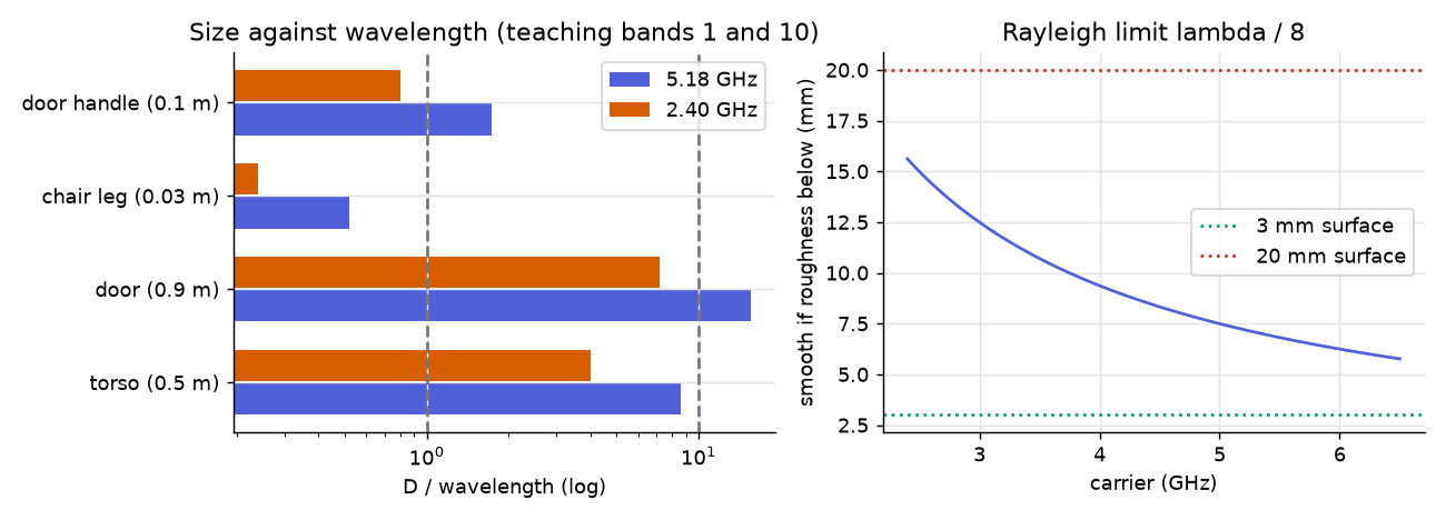
Concept check. Why is a chair leg invisible to a ray tracer at 5 GHz, but a wall is not? Answer: the leg is about one wavelength across (D/λ = 0.52), so the wave diffracts round it; a wall is tens of wavelengths across and its surface is smooth at the wavelength scale.
2 · The image method: scene in, path list out
In a rectangular room every specular path is a straight line from a mirror image of the transmitter to the receiver.
Derivation. A reflection off a wall preserves the path length: the bounce point B on the wall satisfies |TX−B| = |TX′−B|, where TX′ is the mirror image of TX across the wall. So the length of the bounced path TX→B→RX equals |TX′−RX|, a straight line. The image across x = 0 is (−x, y); across x = W it is (2W − x, y). Images of images continue the lattice. Along x the images are 2iW + x (crossing |2i| walls) and 2iW − x (crossing |2i − 1| walls), the same along y; a path of order n keeps the images whose wall crossings sum to n.
In words: each dot outside the room is a mirror transmitter; its straight line to the receiver, folded back at the walls, is one bounce path. Geometry sets lengths and delays; the material enters only through Γ.
Path count in 2-D: order n has 4n paths, so up to depth n_max there are 1 + 4(1 + 2 + … + n_max) = 1 + 2n_max(n_max + 1). The workbook counts 1, 5, 13, 25, 41 for n_max = 0 to 4.
The n_max = 1 path table (Γ = 0.40):
| path | length (m) | delay (ns) | amplitude (dB) |
|---|---|---|---|
| line of sight | 10.00 | 33.36 | −20.0 |
| bounce off y = 0 | 11.31 | 37.74 | −29.0 |
| bounce off y = 8 | 11.31 | 37.74 | −29.0 |
| bounce off x = 0 | 13.42 | 44.75 | −30.5 |
| bounce off x = 12 | 13.42 | 44.75 | −30.5 |
Check one row by hand. The bounce off the wall y = 0 uses the image (2, −1). Its offset to the receiver is (10 − 2, 7 − (−1)) = (8, 8), so d = √128 = 11.3137 m. Then a = 0.40¹/11.3137 = 0.03536, 20 log₁₀ 0.03536 = −29.03 dB, and τ = 11.3137/2.998·10⁸ = 37.74 ns. The workbook prints the same three numbers. The habit to keep: before trusting a tool's path list, recompute one row by hand.
The folded polylines used for drawing reproduce every path length: over all 25 paths at n_max = 3 the largest difference between the folded length and the image distance is 0.0 m (to 12 decimals).
Break it: at n_max = 4 the room has 41 paths. With Γ = 0 only the line of sight survives at any depth (the workbook counts one non-zero path at n_max = 4).
A production tracer finds candidate paths by exhaustive search or by shooting rays from a Fibonacci lattice, then applies the image method to each candidate (hoydis2023_7aa4 ↗). Mirroring sensors on walls to predict echo-path lengths and delays is also used in device-free localisation (cimdins2022_fc11 ↗).
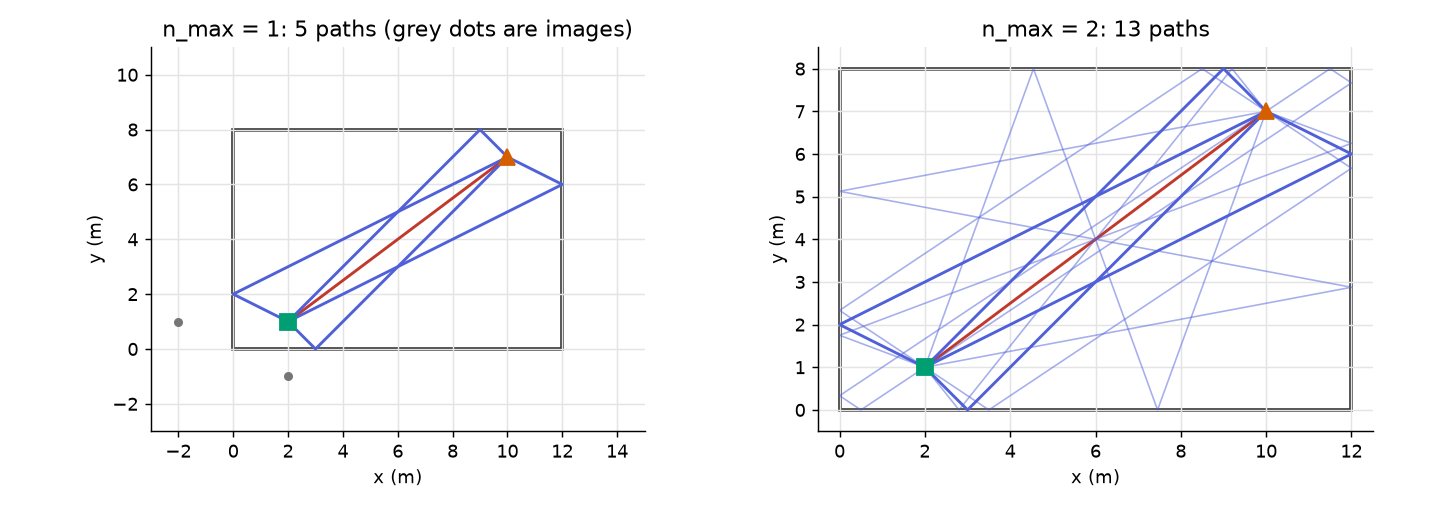
Concept check. How many paths does the room have at n_max = 3, and how many of them are third-order? Answer: 1 + 2·3·4 = 25 paths, of which 4·3 = 12 are third-order.
3 · Why the sum ripples: two paths
The antenna sums fields, so each path is a phasor aₖ e^(−j2πfτₖ). For two paths of relative amplitude r = a₂/a₁ and length difference Δd:
The cosine repeats every Δf = c/Δd in frequency, and its depth is set by r alone:
In words: as frequency rises the second arrow turns against the first; the channel is loud where they line up and quiet where they oppose. CSI is the room's path-length differences written across the tones.
Worked numbers. Δd = 1.31 m gives a 228.8 MHz beat, so an 80 MHz channel sees 0.35 of one cycle; Δd = 3.42 m gives 87.7 MHz and 0.91 cycles; Δd = 1.5 m gives 199.9 MHz. On the 256-tone grid at r = 0.35 and Δd = 1.31 m the in-band ripple is 5.14 dB (maximum +1.40, minimum −3.74 dB relative to a₁), against the 6.35 dB of a full cycle. It is 1.85 dB in a 20 MHz channel and 3.44 dB in a 40 MHz channel: a narrow channel sees only a slice of the beat.
Break it: as r → 1 the trough goes to zero. At r = 0.99 the full-cycle ripple is 45.98 dB; at r = 1 it is infinite, and a display must clamp it ("−∞ dB, perfect null") and never print NaN. As Δd → 0 the in-band ripple is 0.00 dB: the channel is flat, with no frequency structure left to sense.
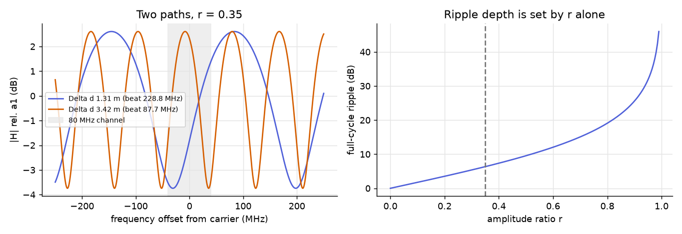
Concept check. Two paths differ by 1.5 m. What is the beat period, and how many cycles fit in 80 MHz? Answer: 2.998·10⁸/1.5 = 199.9 MHz; 80/199.9 = 0.40 cycles.
4 · Many paths: ripple, delay spread, coherence bandwidth, and the depth you truncate at
The full ray sum over the tones:
Here τ̄ is the power-weighted mean delay. The RMS delay spread is the power-weighted standard deviation of excess delay, and the coherence bandwidth is proportional to its inverse (bensky2019_6c00 ↗). The constant 1/(2π) is a convention; the reciprocal is physics. The 802.11ac 80 MHz layout has 256 sub-channels, and a Nexmon extractor returns 242 data tones (meneghello2023_0a93 ↗); the widget and workbook use all 256.
In words: the wider the spread of arrival times, the faster the pattern changes across the tones.
Default room (Γ = 0.40, n_max = 1, 5 paths): ripple = −16.61 − (−27.11) = 10.50 dB, τ_rms = 3.84 ns, B_c = 1/(2π·3.84·10⁻⁹) = 41.4 MHz. The ripple depends on the channel width: 0.75 dB in 20 MHz, 2.30 dB in 40 MHz, 10.50 dB in 80 MHz. The total power Σa² is −18.45 dB against −20.00 dB for the line of sight alone. These delays (at most 11.4 ns of excess delay) sit far below the 40 to 800 ns range of measured multipath delays in factories and buildings reported in the same text; this toy is a small empty room, not a cluttered one.
Truncation depth. A tracer stops at a maximum depth n_max. Whether that matters depends on Γ.
| Γ | n_max | paths | ripple (dB) | τ_rms (ns) | B_c (MHz) | total power (dB) | vs n_max = 4 (dB) |
|---|---|---|---|---|---|---|---|
| 0.4 | 0 | 1 | 0.00 | 0.00 | ∞ (flat) | −20.00 | −1.82 |
| 0.4 | 1 | 5 | 10.50 | 3.84 | 41.4 | −18.45 | −0.27 |
| 0.4 | 2 | 13 | 5.70 | 5.98 | 26.6 | −18.21 | −0.03 |
| 0.4 | 3 | 25 | 9.40 | 6.81 | 23.4 | −18.19 | 0.00 |
| 0.4 | 4 | 41 | 8.98 | 7.05 | 22.6 | −18.18 | 0.00 |
| 0.9 | 1 | 5 | 8.02 | 4.44 | 35.9 | −15.00 | −3.60 |
| 0.9 | 2 | 13 | 9.74 | 10.88 | 14.6 | −12.81 | −1.42 |
| 0.9 | 3 | 25 | 15.10 | 17.58 | 9.1 | −11.86 | −0.47 |
| 0.9 | 4 | 41 | 17.08 | 23.82 | 6.7 | −11.40 | 0.00 |
In a lossy room (Γ = 0.4) n_max = 1 already holds all but 0.27 dB of the n_max = 4 power. In a reflective room (Γ = 0.9) n_max = 1 misses 3.60 dB, and τ_rms keeps growing from 4.44 ns to 23.82 ns while B_c falls from 35.9 to 6.7 MHz. The ripple is not monotone in n_max (Γ = 0.4: 10.50, 5.70, 9.40, 8.98 dB): adding a path changes the phasor sum, not just its size. The truncation depth is part of the instrument, not a detail. At n_max = 0, τ_rms = 0 and B_c is infinite; a display must show "∞ (flat)", not Infinity.
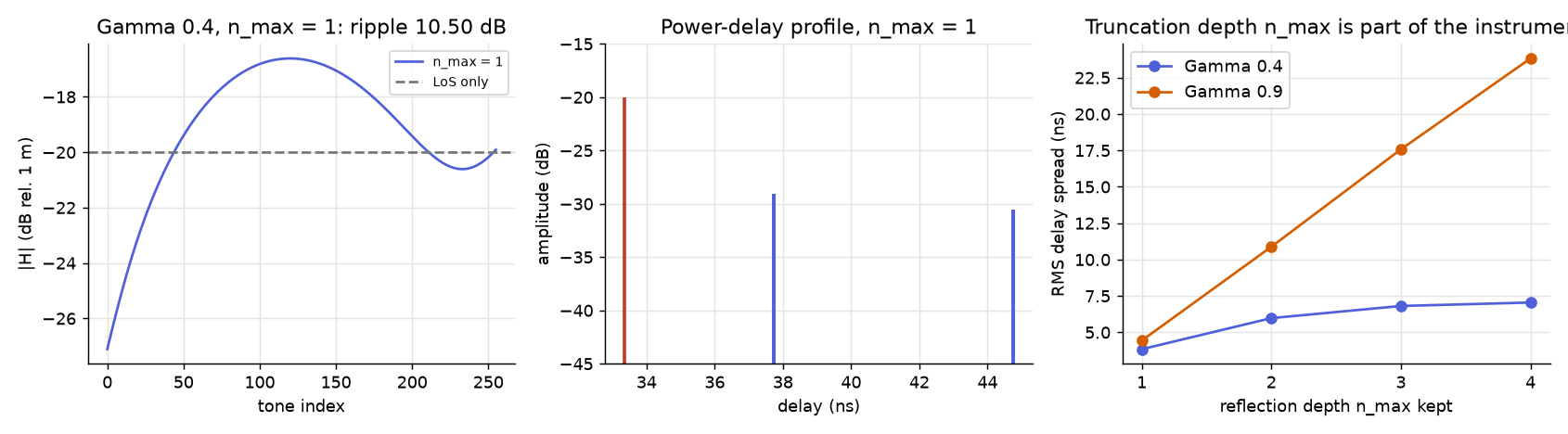
Concept check. A colleague says "n_max = 1 is enough, the extra paths are 30 dB down". When is she right? Answer: when Γ is small: at Γ = 0.4 the missing power is 0.27 dB and τ_rms differs by 3.2 ns. Not at Γ = 0.9, where n_max = 1 misses 3.60 dB of power and 19.4 ns of delay spread.
5 · A body on the link: the step measures path multiplicity
A body is a lossy disc of radius 0.275 m (a 0.55 m width, the knife-edge width Rampa et al. use for a person, rampa2022_ca57 ↗) with a 0.10 m cosine taper at its edge. A path whose nearest point to the body centre is within the radius is blocked, and its amplitude is multiplied by the body pass factor η, a loss of −20 log₁₀ η dB; between 0.275 and 0.375 m the loss in dB follows half a cosine down to zero. With mₖ bodies on path k:
In words: the person removed one arrow from the sum; what is left decides how deep the dent is.
The step depends on how many paths the body blocks. At η = 0.3 the loss per blocked path is 10.46 dB. The unoccluded level at f₀ is −16.64 dB.
| track | body position | paths blocked | step at η = 0.3 |
|---|---|---|---|
| mid-room (x = 6 m, y from 1 to 7 m) | (6, 4.0), on the line of sight | 1 of 5 | −16.64 → −21.26: 4.61 dB |
| near receiver (x = 9.85 m, y from 4.0 to 7.9 m) | (9.85, 6.8875), on the line of sight | 5 of 5 | 10.46 dB, the per-path loss exactly |
Mid-room the body blocks the line of sight only, and the four reflections fill the shadow. Near the receiver the body centre is 0.19 m from the antenna (d₂ = 0.1875 m), inside the body's own 0.275 m radius, so all five paths converge into the body's footprint, so every term is scaled by η and the step equals the per-path loss. The steps for three pass factors (at the default point; the maximum along the whole track is identical to two decimals):
| η | loss per path (dB) | mid-room step (dB) | near-receiver step (dB) |
|---|---|---|---|
| 0.1 | 20.00 | 6.17 | 20.00 |
| 0.3 | 10.46 | 4.61 | 10.46 |
| 0.7 | 3.10 | 1.78 | 3.10 |
Break it: at η = 0.1 the same body is a 6.17 dB dent mid-room and a 20 dB hole near the receiver. Whether it looks transparent or opaque is a fact about the geometry as much as about the body. A review of Bluetooth-based passive sensing reports about 10 dB of attenuation when a human body occludes the 2.4 GHz line of sight, citing a 2014 experiment (iannizzotto2022_1c98 ↗, a secondary report); the default η = 0.3 (10.46 dB) is chosen to sit at that figure, and the range 0.1 to 0.7 brackets it.
Fresnel radius. The first Fresnel zone of a link is the ellipsoid of points P for which the detour TX → P → RX is at most half a wavelength longer than the direct path. Its radius at a point d₁ from one end and d₂ from the other is
Mid-link on the 10 m line of sight: r₁ = √(0.0579·5·5/10) = 0.380 m. Near the receiver (d₁ = 9.8125 m, d₂ = 0.1875 m): r₁ = 0.103 m. A body of radius 0.275 m underfills the zone mid-link and overfills it near the antenna, which is why the same body behaves so differently. Twice the mid-link radius, 0.76 m, is consistent with the maximum first-zone diameter of 0.77 m quoted for 5 GHz over 10 m (wang2025_2c42 ↗, who also report that more than 70 % of the signal energy passes through the first zone). For a related zone model applied to CSI see wu2022_75d3 ↗.
The body model is deliberately simple: a lossy disc, not an electromagnetic solution. The multibody knife-edge model in the literature tracks field RSSI with an average error of about 4 dB (rampa2022_ca57 ↗); no such accuracy is claimed for this disc.
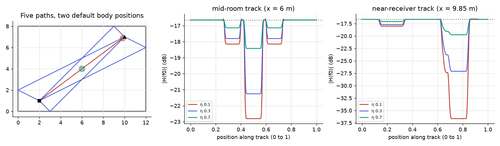
Concept check. Why is the mid-room dent at η = 0.3 (4.61 dB) less than half the per-path loss (10.46 dB)? Answer: the body blocks one of five paths; the other four terms of the sum are untouched and partly fill the shadow, so the step reflects how many terms were removed and how large they were.
6 · A crowd is a falling Rician K
The Rician K factor is the ratio of power in the direct path to power in the scattered paths (ma2020_4782 ↗; Rice parameter ν² = KΩ/(1 + K), with Ω the total power). With N bodies the channel splits into a deterministic part (the traced paths, each blocked by whoever stands on it) and a diffuse part (weak scattering off each body with effectively random phase):
The scatter amplitude is the bistatic radar equation in the 1 m free-space convention; d_TX is the distance from the transmitter to the body and d_RX from the body to the receiver. The scatter cross-section σ is an assumption (default 1 m²): the corpus gives no number for a human body at Wi-Fi frequencies, and the only related hit says that only coarse measured estimates exist.
Derivation of the trend. Two mechanisms act as N grows.
- Diffuse powers add, so P_diff ∝ N, which subtracts 10 log₁₀ N from K. That term is concave in N.
- Each body independently blocks a given path with a small probability p and, when it does, leaves a power fraction β = η² (0.09 at η = 0.3). The deterministic power decays as
a straight line in dB with slope −4.34·p(1 − β) dB per person.
Together, K_dB(N) ≈ K₀ − 10 log₁₀ N − cN, near-linear over moderate N. In words: each extra person adds scatter and may stand on a path; both push the steady part down relative to the random part.
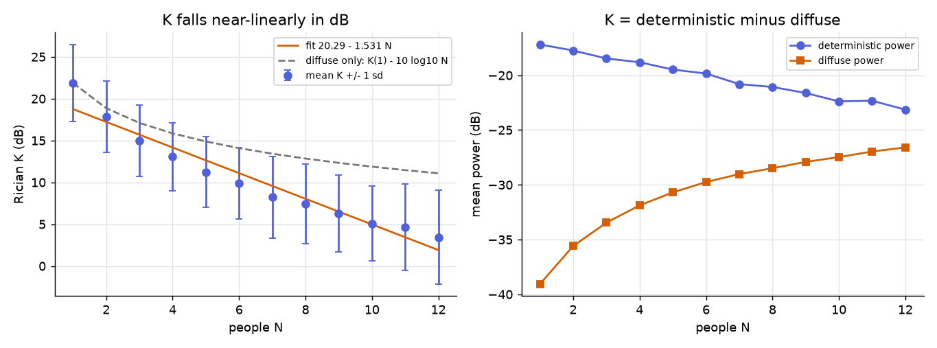
Monte Carlo. 300 seeded placements per N for N = 1 to 12, bodies uniform in [0.3, W − 0.3] × [0.3, L − 0.3] and rejected within 0.6 m of either antenna, η = 0.3, σ = 1 m². The generator is mulberry32(7), seeded once at the start, with x then y drawn per placement (a rejected body consumes both draws); the workbook ports it bit for bit from the deck's JavaScript (the first two draws are 0.01170475 and 0.06195826).
| N | 1 | 2 | 3 | 4 | 5 | 6 | 7 | 8 | 9 | 10 | 11 | 12 |
|---|---|---|---|---|---|---|---|---|---|---|---|---|
| mean K (dB) | 21.87 | 17.86 | 14.99 | 13.07 | 11.21 | 9.91 | 8.22 | 7.42 | 6.29 | 5.09 | 4.64 | 3.45 |
| sd (dB) | 4.60 | 4.27 | 4.27 | 4.05 | 4.23 | 4.27 | 4.87 | 4.73 | 4.62 | 4.46 | 5.20 | 5.60 |
Straight-line fit: K_dB = 20.29 − 1.531·N, R² = 0.940. The diffuse-only curve K(1) − 10 log₁₀ N reaches 11.08 dB at N = 12, against 3.45 dB measured: the deterministic decay supplies the rest.
The two parts can be read separately, because K in dB is the deterministic power in dB minus the diffuse power in dB, so their slopes add. The deterministic power falls 0.538 dB per person (a linear fit) and the diffuse power rises 0.993 dB per person; 0.538 + 0.993 = 1.531. The simple estimate of blocking uses only the line of sight: p ≈ 2·0.275·10/((12 − 0.6)(8 − 0.6)) = 0.065, a decay of 0.27 dB per person. That is half the measured 0.538 dB. The estimate ignores the taper, the four reflected paths and the change of phasor sum when one term is removed, so it gives the order of magnitude and not the value.
Break it, three ways.
- Change σ: it shifts K rigidly and leaves the slope alone. With η = 0.7 and σ = 2 m² the fit is K₀ = 17.33 dB, slope 1.201; with σ = 0.3 m² it is K₀ = 25.57 dB and the same slope 1.201. The intercepts differ by 8.24 dB = 10 log₁₀(2/0.3). The slope is set by η (through blocking), the level by σ.
- Change η: from 0.3 to 0.7 the slope drops from 1.531 to 1.201 dB per person, because a weaker body blocks less.
- Use fewer placements: with 50 placements per N and seeds 7, 8, 9 the slope is 1.525, 1.555, 1.575 (300 placements: 1.531) and the mean K at N = 4 is 13.46, 14.14, 11.76 dB (300 placements: 13.07). The slope is an estimate with Monte Carlo error; the mean at a single N moves by about ±1.2 dB.
The slope is a property of this room and these constants, not a physical constant. The corpus holds no paper that measures K against crowd count; the schedule above is derived from independent blockers and scatterers, not cited. A qualitative report that the CSI amplitude bundle widens as more people walk in the area (choi2022_17c2 ↗) points the same way and gives no K.
Note the size of the spread against the trend: the per-N standard deviation is 4.0 to 5.6 dB, while adjacent N differ by about 1.5 dB. Three extra people (4.6 dB) is about one standard deviation, so a single snapshot of K does not identify N; the trend is a statement about the ensemble.
Concept check. Doubling σ from 1 to 2 m² changes the fitted K₀ by how much, and the slope by how much? Answer: K₀ falls by 10 log₁₀ 2 = 3.01 dB and the slope does not change, because P_diff scales linearly with σ and the blocking term does not depend on it.
7 · Channel-relative diffuse power, and the setting that makes the simulator inert
The diffuse overlay needs a power level. Two ways to set it.
- Absolute: one table value for every link.
- Channel-relative: the overlay of each link is a fraction of that link's own traced power,
In words: if the random part is set relative to each link, changing the walls still changes what the receiver sees; if it is one loud number for every link, the walls stop mattering.
Links in a building spread over tens of dB. An absolute level loud enough to matter on a strong link buries the weak ones, and once the observation is dominated by the overlay a change of wall material no longer moves it.
A two-link toy. Link A is the default receiver: line of sight plus the four first-order wall paths. Link B is a farther receiver at (11.5, 7.5) m whose line of sight is blocked by a cabinet, so it holds only the four wall paths; it is 3.82 dB weaker than A. Two materials: concrete (Γ = 0.40) and metal (Γ = 0.95). The observed envelope is √(|H_det|² + P_diff), and the material sensitivity is
over the 256 tones, for concrete (c) against metal (m). With the defaults k₀ = 16 dB, s = 1.5 dB per person, N = 4: K_dB = 16 − 1.5·4 = 10 dB, K = 10.0, and P_diff = 0.100·P_det.
| overlay | link A | link B |
|---|---|---|
| none (deterministic) | 0.792 | 1.375 |
| channel-relative, K = 10 dB | 0.771 | 1.375 |
| channel-relative, K = 6 dB | 0.750 | 1.375 |
| absolute, +0 dB over link A | 0.446 | 0.546 |
| absolute, +20 dB | 0.0111 | 0.0103 |
| absolute, +40 dB | 1.13·10⁻⁴ | 1.04·10⁻⁴ |
| absolute, +80 dB | 1.13·10⁻⁸ | 1.04·10⁻⁸ |
The overlay sits X + 3.8 dB above link B when it sits X dB above link A (23.8 dB at X = 20).
Why the absolute overlay kills sensitivity. With a constant overlay P ≫ |H|², the envelope is √(P + |H|²) ≈ √P + |H|²/(2√P). The difference between two materials is (|H_c|² − |H_m|²)/(2√P), and the norm of the envelope is about √P times √256, so rel-L2 ∝ 1/P: one decade of rel-L2 per 10 dB of overlay. The table follows it exactly (0.0111 at +20 dB, 1.13·10⁻⁴ at +40, 1.13·10⁻⁸ at +80). The channel-relative form keeps the ratio of overlay to signal fixed, so the material contrast survives.
Scale invariance. Add a through-wall loss of 30 or 60 dB to every link-B path. In channel-relative mode the link-B rel-L2 stays 1.375 at 0, 30 and 60 dB (everything scales together). In absolute mode (X = 20) it falls from 0.0103 to 1.04·10⁻⁵ at 30 dB and 1.04·10⁻⁸ at 60 dB, where the overlay sits 83.8 dB above link B. A building's link budget spans that range; an absolute level cannot be right for all of it.
A real instance. In a ray-traced simulation of a multi-room building floor, an occupancy overlay was specified as an absolute power (level 35, in the simulator's power units). It sat about 80 dB above the traced power of a link: 10 log₁₀(35/2.76·10⁻⁷) = 81 dB, using the per-link traced power (2.76·10⁻⁷) logged after the repair. Swapping every wall from concrete to metal produced byte-identical output: the same output variance statistic (log-variance 1.1177) and the same mean |H| of 8.18. The overlay was the output; the traced channel was not in it. After re-specifying the overlay as |H_det|²/K(N), the same swap changed the output: rel-L2 0.49, ratio of mean |H| 0.84, and the logged diffuse-to-deterministic power ratio matched 1/K (1.74·10⁻⁷/2.76·10⁻⁷ = 0.63 against 1/1.58 = 0.633 for the logged mean K of 1.58). This instance is a single case reported from the lab's own simulator, not a benchmark; the corpus is silent on how a ray tracer's diffuse overlay should be parameterised.
Lesson. A simulator's most dangerous state is inert, not wrong. A wrong simulator disagrees with something; an inert one agrees with itself. Every sweep needs one comparison whose sign you can predict, so that its absence raises an alarm. Here the prediction is: replacing concrete by metal raises the mean received power of link A by 4.57 dB in the deterministic channel; if the observed output does not move at all, the overlay has swamped the scene.
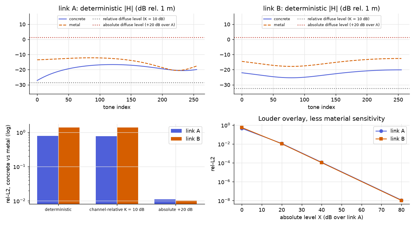
Concept check. An absolute overlay is set 20 dB above the median link. What happens to a link 30 dB weaker than the median? Answer: the overlay sits 50 dB above it and its material sensitivity is about 10⁻⁵ (the workbook's 30 dB through-wall case: 1.04·10⁻⁵), effectively inert; the strongest links may still respond weakly (0.011 at +20 dB).
8 · Calibrating the scene: differentiable tracing and a truncated model
A tracer's output is only as good as its scene, and material properties are the hardest part to obtain. Sionna RT is differentiable with respect to material properties, positions and antenna patterns, so materials can be fitted to channels by gradient descent. Hoydis et al. recover four materials of a city scene from 400 receivers (128 subcarriers at 30 kHz spacing, initial σ = 0.1 S/m and εr = 3.0) after about 100 iterations; wood converges slowly because few paths touch it (hoydis2023_7aa4 ↗). They add two cautions: training on complex CFRs is unlikely to work well with measured data, since accurate phase can rarely be predicted by ray tracing, and the goal is not necessarily the correct material but the one that best predicts the measured channel with the chosen tracer, a calibration of the tracer and environment model.
The trap: a model that omits physics absorbs the error into the parameter it is allowed to move.
A toy. The truth is generated with Γ* = 0.60 at n_max = 3 in the default room. We fit Γ by grid search over linspace(0, 0.95, 951) with a model of a chosen depth n_max. Because a path of order n scales with Γⁿ, the model is a polynomial in Γ:
In words: the curve shows how wrong the simulated channel is for each wall guess; its lowest point is the material the fit reports.
| model n_max | complex CFR: best Γ | NMSE (dB) | magnitude only: best Γ | NMSE (dB) |
|---|---|---|---|---|
| 1 | 0.330 | −2.4 | 0.000 | −6.5 |
| 2 | 0.598 | −9.1 | 0.610 | −13.3 |
| 3 | 0.600 | exact (−300, the clamp) | 0.600 | exact |
| 4 | 0.591 | −16.9 | 0.597 | −19.8 |
The n_max = 3 model recovers the truth exactly because it is the truth. n_max = 2 recovers 0.598 with a residual of −9.1 dB, so the small error is visible in the loss and the material looks right. n_max = 1 fits the complex CFR to 0.330 and the magnitude to 0.000 (a line-of-sight-only model): the fit converges confidently to a wrong wall, with the loss at the true Γ of only −1.6 dB. n_max = 4 overshoots the truth model and lands at 0.591 and 0.597. A fitted material is a statement about model plus scene, not about the wall.
The depth-truncation bias in calibration is not discussed in the corpus; the toy demonstrates it and is not a literature result.
What a clean tracer can and cannot say. Sort every claim into one of three bins.
- Derived: follows from the equations (the beat period, the K trend's form, the rel-L2 scaling).
- In silico: holds in this simulator with these constants (the K slope of 1.531, the body step of 4.61 dB).
- Measured: needs a measurement to stand (a material's Γ, a body's η and σ, the accuracy of a path list).
A clean ray tracer is structure and sensitivity evidence: which paths exist, which a body occludes, how a change in one parameter moves the output. Its accuracy against the world has to be shown with measurements, and the corpus holds no published comparison of ray-traced indoor CSI against measured CSI.
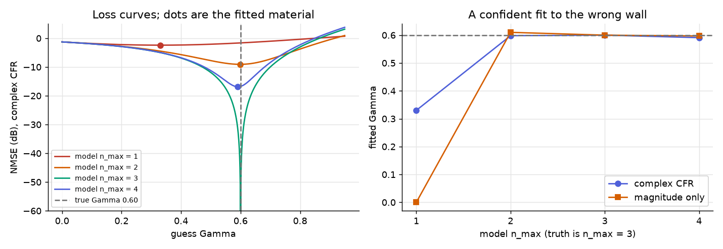
Concept check. Why does an n_max = 1 model fit the complex CFR to Γ = 0.330 and not to 0.60? Answer: the truth holds higher-order terms Γ² and Γ³ that the model lacks; the fit lowers Γ to make the first-order terms mimic what the missing paths add, and the residual (−2.4 dB) is the price.
Exam questions
Q1 · Derivation. Two paths of amplitude a₁ and a₂ = r·a₁ differ in length by Δd. Derive the frequency pattern of |H|, its period and its depth. For Δd = 1.5 m and r = 0.35, give the period, the number of cycles in an 80 MHz channel and the full-cycle ripple. Model answer. H = a₁ + a₂e^(−j2πfΔd/c) up to a common phase, so |H|² = a₁²(1 + r² + 2r cos(2πfΔd/c)). The cosine repeats when fΔd/c changes by 1: Δf = c/Δd = 2.998·10⁸/1.5 = 199.9 MHz, so an 80 MHz channel holds 80/199.9 = 0.40 cycles. Peak to trough: 20 log₁₀((1 + r)/(1 − r)) = 20 log₁₀(1.35/0.65) = 6.35 dB, set by r alone. The period is set by the geometry alone.
Q2 · Truncation. A tracer is configured with n_max = 1 for a room with Γ = 0.9 instead of Γ = 0.4. What changes in the quality of the answer, with numbers? Model answer. At Γ = 0.4 n_max = 1 holds all but 0.27 dB of the n_max = 4 power and τ_rms is 3.84 ns against 7.05 ns. At Γ = 0.9 n_max = 1 misses 3.60 dB, and τ_rms is 4.44 ns against 23.82 ns at n_max = 4; B_c would be reported as 35.9 MHz instead of 6.7 MHz. Each bounce multiplies a path by Γ, so a reflective room carries power in high orders. The truncation depth belongs to the instrument description and must be reported with any result.
Q3 · Body step. A body with pass factor 0.3 crosses a link. Explain why the amplitude dent is 4.61 dB when the body is in mid-room on the line of sight and 10.46 dB when it stands on the line of sight 0.19 m from the receiver. Model answer. Blocked paths are scaled by η, a loss of 20 log₁₀(1/0.3) = 10.46 dB each. Mid-room the body stands on one of five paths (the line of sight) and the four reflections, unblocked, remain in the sum: the step is 4.61 dB. Near the receiver all five paths pass through the body's footprint, every term is scaled by 0.3, and the step equals the per-path loss. First Fresnel radius: 0.380 m mid-link against 0.103 m near the receiver, so a 0.275 m body underfills the zone in one place and overfills it in the other. The step measures how many terms were removed, not how opaque the body is.
Q4 · K against crowd size. Derive why K in dB is near-linear in N, name the two mechanisms, and say what sets the slope and what sets the level in the simulation of section 6. Model answer. Independent scatterers add diffuse power, P_diff ∝ N, so K loses 10 log₁₀ N (concave). Independent blockers each remove a path with small probability p, leaving a fraction β of its power, so deterministic power decays as (1 − p(1 − β))^N ≈ e^(−p(1−β)N): a straight line in dB. K_dB ≈ K₀ − 10 log₁₀ N − cN. In the executed run K_dB = 20.29 − 1.531·N (R² = 0.940), with the deterministic part contributing 0.538 dB per person and the diffuse part 0.993. The level is set by the scatter cross-section σ (K₀ shifts by 10 log₁₀ of its ratio: 8.24 dB between 0.3 and 2 m²) and the slope by the pass factor η (1.531 at 0.3, 1.201 at 0.7). The constants are assumptions and the slope is a property of this room; the corpus has no measurement of K against N.
Q5 · A partial failure. A team sets its diffuse overlay as one absolute level equal to the power of the median link (X = 0 dB in the two-link toy). Their material sweep still moves the output. Are they safe? Model answer. Not safe, only less blind. At X = 0 dB the rel-L2 between concrete and metal is 0.446 on link A and 0.546 on link B, against 0.792 and 1.375 for the deterministic channel and 0.771 and 1.375 for a channel-relative overlay at K = 10 dB: the sensitivity is cut to 56 % on link A and 40 % on link B, and it falls by a factor of 10 for every 10 dB by which a link lies below the level (rel-L2 ∝ 1/P). Weak links in a real building, 30 to 60 dB down, are inert (1.04·10⁻⁵ at 30 dB, 1.04·10⁻⁸ at 60 dB in the toy). The check that would catch it is a sweep comparison with a predictable sign, evaluated per link and not on the average.
Q6 · What does a calibrated fit say? An n_max = 1 tracer fitted to a channel yields Γ = 0.33 with a final NMSE of −2.4 dB. The team reports "the wall has Γ = 0.33". Criticise. Model answer. In the toy the truth is Γ = 0.60 with three orders of reflection. An n_max = 1 model absorbs the missing paths into the parameter and converges to 0.330 (0.000 if only magnitudes are fitted). The fitted value is a statement about model plus scene: it is the value that makes this truncated tracer best imitate the channel, which is what Hoydis et al. call a calibration of the tracer and environment model, not a wall measurement. To make a claim about the wall the model must contain the physics that matters (here, depth), or the claim must be tested against measurements the model was not fitted to. The corpus holds no published comparison of ray-traced indoor CSI against measured CSI.
Where this goes next
A body that moves changes path lengths over time. The stage that turns a trajectory into a sequence of ray sums is a data contract (metres, seconds, a frame clock), and the per-path phase rate 2v/λ (the Doppler shift) is why the frame rate matters. The names and units kept from this week are the body pass factor η (0.1 to 0.7, an amplitude multiplier per blocked path), the scatter cross-section σ (0.3 to 2 m², amplitude √(σ/4π)/(d_TX·d_RX)), the carrier (2.4 to 6.5 GHz) and the 1 m free-space dB convention. The channel here is noiseless and perfectly synchronised; the receiver's noise, clock and gain control come in a later week. The calibration break of section 8 and the "clean tracer is structure and sensitivity evidence" rule prepare the calibration and validation weeks.
Further reading
- hoydis2023_7aa4 ↗: the image method inside a production tracer, Fibonacci ray shooting and differentiable material learning.
- zhang2024_df4a ↗: 4 interactions, 100,000 rays, the λ/8 roughness rule, frequency-selective fading.
- rampa2022_ca57 ↗: the knife-edge body, 0.55 m width, Fresnel radius, about 4 dB model error.
- wang2025_2c42 ↗: the first Fresnel zone, energy share and size at 5 GHz.
- wu2022_75d3 ↗: further reading on Fresnel zones.
- iannizzotto2022_1c98 ↗: the roughly 10 dB body occlusion at 2.4 GHz (secondary report).
- ma2020_4782 ↗: the Rician K definition.
- bensky2019_6c00 ↗: delay spread, coherence bandwidth, knife-edge diffraction, Rayleigh against Rician.
- meneghello2023_0a93 ↗: 256 sub-channels, 242 data tones at 80 MHz.
- cimdins2022_fc11 ↗: the image method in device-free localisation.
- choi2022_17c2 ↗: qualitative growth of the CSI amplitude bundle with the number of people.
Provenance (instructor only)
Executed sources, vault paths:
- obsidian/monad-knowledge/edu/courses/SIM507-simulation-toolkits/week-03-ray-traced-channel-simulation/workbook.ipynb
- obsidian/monad-knowledge/edu/courses/SIM507-simulation-toolkits/week-03-ray-traced-channel-simulation/numbers.json
First-party numbers (section 7, "A real instance"):
- obsidian/monad-knowledge/experiments/campaigns/c-cac-drift.md (lines 79 to 94: absolute overlay level 35, byte-identical concrete and metal output with log-variance 1.1177 and |H| 8.18, rel-L2 0.49 and |H| ratio 0.84 after the change, logged powers 2.76e-7 and 1.74e-7, mean K 1.58). Caveat: the note's own statement "|H_det| about 1e-4" does not give 80 dB against an amplitude of 5.9 (that would be about 95 dB); the 80 dB matches the power form, 10 log₁₀(35/2.76e-7) = 81 dB, which is what the lecture quotes. The per-link power 2.76e-7 is logged after the repair, so the 81 dB is an estimate of the pre-repair gap, not a measurement of it.
Literature notes (where each cited figure sits):
- literature/Sionna RT Differentiable Ray Tracing for Radio Propagation Modeling (hoydis2023_7aa4).md (sections II and III-B: image method, Fibonacci lattice; section III-A: learning radio materials, 400 receivers, 128 subcarriers at 30 kHz, about 100 iterations, remarks on measured data)
- literature/WiSegRT Dataset for Site-Specific Indoor Radio Propagation Modeling with 3D Segmentation and Differentiable Ray-Tracing.md (sections III-A, Table I, II-B: 100,000 rays, 4 interactions, 2.4 GHz, λ/8)
- literature/Electromagnetic Models for Passive Detection and Localization of Multiple Bodies.md (sections IV-A, IV-C: knife-edge width 0.55 m, about 4 dB error)
- literature/Guiding Wi-Fi Sensor Placement for Enhanced CSI-Based Sensing in Stationary Crowd Counting.md (Fresnel zone model: over 70 % of energy, 0.77 m at 5 GHz over 10 m)
- literature/A Perspective on Passive Human Sensing with Bluetooth.md (about 10 dB body occlusion, secondary report)
- literature/WiFi Sensing with Channel State Information.md (Statistical Models: Rician K, ν² = KΩ/(1 + K))
- literature/Short-range Wireless Communication.md (ch. 2.3 and 2.7: delay spread, coherence bandwidth, 40 to 800 ns)
- literature/A CSI Dataset for Wireless Human Sensing on 80 MHz Wi-Fi Channels.md (256 and 242 tones)
- literature/Exploiting Ultra-Wideband Channel Impulse Responses for Device-Free Localization.md (image method for echo paths)
- literature/Wi-CaL WiFi Sensing and Machine Learning Based Device-Free Crowd Counting and Localization.md (qualitative amplitude bundle width)
- literature/WiFi CSI-based device-free sensing from Fresnel zone model to CSI-ratio model.md (further reading only, no number quoted)
Corpus silences and derivations:
- No published comparison of ray-traced indoor CSI against measured CSI.
- No corpus paper measures the Rician K factor against crowd count; the linear-in-dB schedule is derived, not cited.
- No numeric radar cross-section of a human body at Wi-Fi frequencies (only a statement that coarse measured estimates exist); σ = 1 m² is an assumption.
- Nothing on parameterising a diffuse overlay absolutely versus relative to the specular channel; the mechanism is taught from first principles plus one first-party instance.
- No numeric validity threshold for geometric optics in terms of D/λ; the bands in section 1 are a teaching rule of thumb, the Rayleigh λ/8 rule is the only quantitative criterion.
- Depth-truncation bias in material calibration is not discussed in the corpus; the section 8 toy demonstrates it.
- The pass factor default η = 0.3 is chosen to match the roughly 10 dB literature figure, which is a secondary report of a 2014 experiment; the body disc, taper (0.10 m) and the bodies' placement region are modelling choices of this week.