This note is the reader companion to the deck. It follows the deck's order. Every worked number comes from the executed workbook (workbook.ipynb, all scalars in numbers.json). Each concept in the deck is a live widget; the numbers below are what the widget shows at its default state.
0. Why this week exists
A survey of more than 1,500 scientists is reported, at second hand, to have found that 70 % had tried and failed to reproduce earlier results; the primary survey is not in the corpus, so the figure is a secondary report (pride2025_51f1 ↗, related work). The same paper argues for archiving code, parameters, dependencies and environment. A simulator is cheap to re-run, so for a simulator the failure is a choice: nothing forces us to lose the inputs.
Six words carry the week.
- Simulator: a program that imitates a piece of reality so an idea can be tested.
- Run: one execution with one specific set of inputs.
- Artefact: a file a run leaves behind.
- Manifest: the run's packing list, describing the inputs and the artefacts.
- Seed: an integer that starts the random stream.
- Digest: a fixed-length fingerprint of a byte string.
The four kinds of simulator that recur in sensing and crowd research are told apart by what goes in and what comes out. A crowd mover takes a floor and a headcount and returns trajectories. A measurer takes trajectories and returns metrics. A radio tracer takes a scene and trajectories and returns a channel. A notebook takes parameters and returns an executed worksheet. The crowd mover's trajectory feeds the other two. That arrow is why later weeks lean on the same "trajectory artefact".
1. A simulator is a function
Bake a cake with the same recipe, the same ingredients and the same model of oven, and the cake is the same each time. Change any one of the three and the cake changes. Strip the domain away:
In words: the model is the rules, \theta are numbers with units, s is the seed, e is the environment (code version, numeric precision, libraries), and the a_i are a fixed set of files. It is an instrument only if fixing all four inputs fixes the bytes.
The toy used all week: N agents walk a corridor from x = 0,
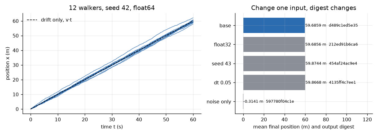
In words: each step adds a drift of v\,\Delta t and a random kick whose size grows like the square root of the step length. The defaults are v = 1.0 m/s, \sigma = 0.2 m/\sqrt{\text{s}}, N = 12, T = 60 s, \Delta t = 0.1 s, seed 42, float64. Z_k comes from the generator of section 2, consumed per step, per agent, u1 then u2.
Worked numbers (workbook section 1). The output digest is the first 12 hex characters of SHA-256 over the final positions in micrometres, comma-joined; rounding to micrometres absorbs one-ulp differences between math libraries.
| Input changed | Mean final position (m) | Output digest | Digest changed |
|---|---|---|---|
| none (base) | 59.6859 | d489c1ed5e35 | |
| model: noise only (v forced to 0) | -0.3141 | 597780f04c1e | yes |
| \theta: v = 1.05 | 62.6859 | 8f984a66f793 | yes |
| seed 43 | 59.8744 | 454af24ac9e4 | yes |
| environment: float32 | 59.6856 | 212ed91b6ca6 | yes |
| \Delta t = 0.05 s (code default) | 59.8668 | 4135ff4c7ee1 | yes |
Running the base inputs twice gives the same digest. The drift alone would give 60 m; the base run is 0.70 standard errors below it (standard error of the mean of 12 agents, 0.2\sqrt{60}/\sqrt{12} = 0.4472 m). The float32 switch moves the mean by 0.0003 m and changes every byte. The environment is an input.
Concept check. Why is the digest taken over micrometres and not over raw floating-point bytes? Because the same arithmetic in two math libraries can differ in the last bit, and the digest is meant to detect a change of input, not a change of libm.
2. Where the randomness comes from
A pseudo-random generator is a deterministic recurrence started from a seed. The multiple-recursive family is X_t = (a_1 X_{t-1} + \dots + a_k X_{t-k}) \bmod m with uniforms U_t = X_t/m (kroese2019_3738, eq. 3.1, Chapter 3). With order k = 1 and no increment it is the multiplicative congruential generator used here:
In words: the seed is the starting row of a fixed table; the recurrence reads the table forward; dividing by m squeezes the integers into (0, 1). The constants a = 16807, m = 2^{31} - 1 are a design choice of this course. The corpus is silent on these constants, on period and lattice tests, and on the weakness below; they are taught from the closed form.
Box-Muller turns two uniforms into a standard normal (kroese2019_3738, Algorithm 3.2.1):
In words: U_1 sets a radius (small U_1, large radius), U_2 sets an angle; the cosine projects the point onto one axis, and the result is bell-shaped.
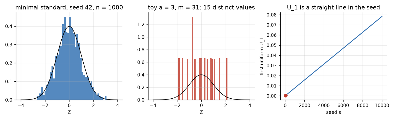
Worked numbers (workbook section 2). Seed 42: X_0 = 43, X_1 = 16807 \cdot 43 = 722701, U_1 = 0.000337, U_2 = 0.656125, Z_1 = \sqrt{-2\ln 0.000337}\cos(2\pi \cdot 0.656125) = -2.2245. The first eight states are 722701, 1409017472, 1054476435, 1550388001, 1952043756, 891731873, 49217098, 410561991. For 1000 normals from seed 42: mean -0.0175, sample sd 1.0080, 1000 distinct values, Kolmogorov-Smirnov statistic 0.0269 (p = 0.456, no departure from N(0,1) detectable). With n = 10{,}000 the mean is -0.0053 and the standard error 0.0100. Seed 43 with n = 1000 gives mean 0.0125.
The period of the minimal standard generator is m - 1 = 2{,}147{,}483{,}646 because a is a primitive root of the prime m; the workbook checks a^{(m-1)/p} \not\equiv 1 for each prime p dividing m - 1.
Break it: a small modulus. With a = 3, m = 31 the period is 30. Two thousand uniforms from seed 42 take 30 distinct values and 1000 normals only 15 distinct values. The mean is 0.0226, the sd 1.1090, both unremarkable; the Kolmogorov-Smirnov statistic is 0.1249 (p below 0.0001). A correct-looking mean does not certify the generator.
Seeds are labels, not randomness. From the recurrence, U_1 = 16807\,(s+1)/m, a straight line in the seed: 0.000008 at s = 0, 0.000337 at s = 42, 0.078264 at s = 9999. Every seed in 0 to 9999 therefore starts with a radius of at least \sqrt{-2\ln 0.078264} = 2.2573; the median first radius over those seeds is 2.5459, against 1.1774 for a truly uniform U_1. First draws of neighbouring small seeds are nearly equal. Section 4 removes this weakness by hashing.
Concept check. State what a seed pins and what it does not. It pins one stream of one generator; it does not pin the true value being estimated, any other stream, or the environment.
3. A seed pins a draw, not the truth
Crude Monte Carlo reports the sample mean with its standard error S/\sqrt{N}, and the approximate interval \bar Y \pm z_{1-\alpha/2}\,S/\sqrt{N} (kroese2019_3738, Section 3.3.1, eq. 3.13). The literature's worked example is \int_0^1 x^3\,dx = 1/4 with N = 10{,}000 uniform draws: estimate 0.248, standard error 0.0028 (wasserman2004_ea08 ↗, Example 24.1). Our generator at seed 42 gives 0.2468 with standard error 0.0028; the exact value is \sqrt{1/7 - 1/16}/100 = 0.0028.
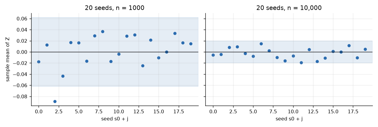
In words: each seed gives a different sample mean; the spread of those means shrinks like 1/\sqrt{n}. The seed chooses which dot you get; n chooses how wide the cloud is.
Worked numbers (workbook section 3). Seeds 42 to 61, n = 1000: S = 1.0080 for seed 42, \mathrm{SE} = 0.0319, band \pm 0.0620. The sd of the 20 means is 0.0308 against the predicted 1/\sqrt{1000} = 0.0316; 19 of 20 means lie inside the band; the range is -0.0891 to 0.0367. With n = 10{,}000 the sd of the 20 means is 0.0098 against 0.0100, and all 20 lie inside \pm 0.0196.
Break it: reuse one seed. Twenty rows with the same seed give one identical mean. The sd is 0.0000 and the strip looks perfectly precise while the evidence is one run (n_{\text{effective}} = 1). Week 7 formalises this as pseudo-replication.
Concept check. Halving the spread of the sample mean needs how many times the samples? Four times, because the spread is \propto 1/\sqrt{n}. Changing the seed never narrows it.
4. One seed, many streams
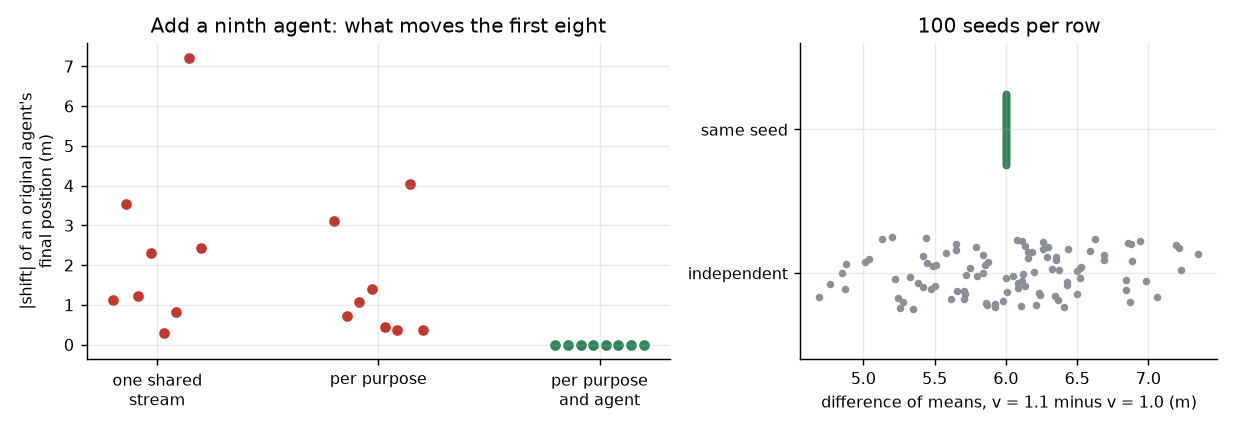
A simulator has several random consumers: start positions, walking noise, arrival times. If they read one shared stream in sequence, adding one agent shifts every later draw, and a comparison of N against N+1 is confounded with a reshuffle of the randomness. Derive one stream per purpose and per entity:
with H the first 8 hex characters of SHA-256 read as an integer. For the key 42|noise|3 the hash prefix is 590b53bb, giving X_0 = 1493914556. In words: give every random choice its own named stream and adding a ninth walker leaves the other eight where they were.
Worked numbers (workbook section 4). Each agent has a start offset x_0 \sim U(0, 2) m; walking as in section 1. Add a ninth agent to eight (seed 42):
| Stream design | Original agents whose path changed | Largest shift of an original final position (m) | Difference of mean final positions, N=9 minus N=8 (m) |
|---|---|---|---|
| one shared stream | 8 of 8 | 7.2186 | -0.9574 |
| one stream per purpose (start, noise) | 8 of 8 | 4.0352 | +0.2035 |
| per purpose and agent (hashed) | 0 of 8 | 0.0 | -0.0394 |
The per-purpose design still fails because the noise stream is interleaved per step and per agent: the ninth agent changes which draw belongs to whom. In the shared design the difference between configurations mixes the effect of the ninth agent with a reshuffle of all the noise. In the hashed design the mean of the original eight is exactly unchanged, so what remains is the ninth walker.
Hashing also repairs the first-draw weakness: over 10,000 keys s|noise|0 the median first radius is 1.1646 (uniform theory 1.1774), against 2.5459 for plain seeds 0 to 9999.
Common random numbers. Comparing two configurations under the same random numbers cannot increase the variance of the difference for continuous marginals; the corpus poses this as an exercise (kroese2019_3738, Chapter 3 exercises). In the toy the noise is additive, so it cancels completely: drift 1.1 against 1.0 over 100 seeds gives a mean difference of 6.0 m with sd 0.000000 m (zero to six decimals) under the same seed, and sd 0.6057 with independent seeds (theory \sqrt{2}\cdot 0.4472 = 0.6325). This is the extreme case; a nonlinear model would show a smaller gain. The corpus is silent on hash-derived or counter-based substreams; the derivation here is a design choice.
Concept check. A run records one seed for "the crowd" and one for "the radio". Why must both be in the manifest? A seed is meaningful only for the stream it pins.
5. The manifest: what a stranger needs to re-run you
Every box leaving a warehouse carries a packing list. A manifest is a run's packing list: model and code version, every parameter with its unit, every seed, the environment, and the artefacts with their roles. A field left out is filled by the re-runner's default, and a default is a guess. One open-source pedestrian simulator writes the Git commit hash into its output files and keeps inputs as human-readable JSON (kleinmeier2019_e6cd ↗). A survey of CSI-sensing datasets grades dependency documentation as complete with exact versions, partial, or absent, and names precisely defined dependencies as essential to replicate the environment (guarino2026_e72c ↗, code availability).
In words: every blank line is a place where the stranger must guess, and one wrong guess is enough.
Teaching assumption (not a literature value): when a field is not recorded the re-runner uses code version 1.1 whose default \Delta t is 0.05 s, a documented default drift of 1.2 m/s, seed 0, float32. When the parameter block is missing, only v differs.
Worked numbers (workbook section 5). The original run is 59.6859 m, digest d489c1ed5e35. Of the 16 combinations of recorded fields, 1 reproduces it (all four recorded). Fields left blank one at a time:
| Blank field | Re-run mean (m) | Re-run digest | Match |
|---|---|---|---|
| code version (\Delta t 0.05 s) | 59.8668 | 4135ff4c7ee1 | no |
| parameters (v 1.2 m/s) | 71.6859 | 700b900351ea | no |
| seed (0) | 60.1893 | 70081bcd1b20 | no |
| environment (float32) | 59.6856 | 212ed91b6ca6 | no |
Three of the four wrong re-runs land within 0.51 m of the original mean, and the float32 one within 0.0003 m. A small numeric difference is not evidence of a faithful re-run.
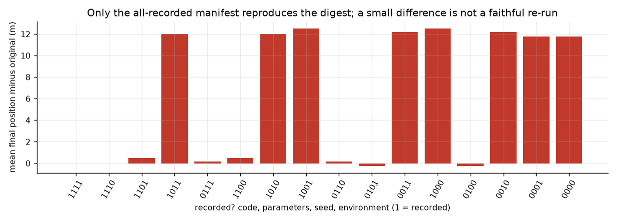
Concept check. Which rows of the table would a mean-only comparison have accepted? A tolerance of 0.51 m on the mean accepts three of the four single-field errors; only the digest rejects all of them.
6. Content digests: naming a run by what it is
A one-way hash maps input of any length to a fixed-length output that is very sensitive to a slight change of input; typical values are 128 bits and longer (dhillon2017_6a80 ↗, preliminaries). The corpus is silent on content-addressed storage, canonical serialisation and SHA-256 itself; the test vector SHA-256("abc") = ba7816bf...f20015ad is checked against Python's hashlib in the workbook.
In words: the digest is a fingerprint of the packing list; change one character and about half the fingerprint changes, change nothing and it is identical to the bit.
The canonical serialisation used here: sorted keys, separators (",", ":"), ASCII, no whitespace. Manifest A is the section 1 default with five artefacts (trajectory, summary, per-bin summary, figure, upstream input) and an image reference that is a teaching string, not a registry. Canonical size 683 bytes; digest starts with 8295ae262ca3b9fb.
Worked numbers (workbook section 6), bits differing from A out of 256:
| Manifest B | Bits differing |
|---|---|
| identical | 0 |
| seed 43 | 121 |
| drift 1.05 | 129 |
| image rebuilt (different digest string) | 125 |
image tag :latest |
119 |
| same content, keys reversed, no canonical serialisation | 130 |
| same content, keys reversed, canonical serialisation | 0 |
Over 999 single-field edits (seeds 0 to 999 except 42) the mean is 127.96 bits, sd 8.03, range 104 to 151, against Binomial(256, 1/2): mean 128, sd 8. The observed distribution is consistent with fair coin flips per bit.
Break it. Without a canonical serialisation, the same content hashes differently under a different key order (130 bits): a false alarm, which is why the serialisation is part of the contract. A tag such as :latest names a moving target: a rebuild behind the same tag leaves the manifest digest identical, because the digest records only the tag string. Week 7 develops this as tag drift.
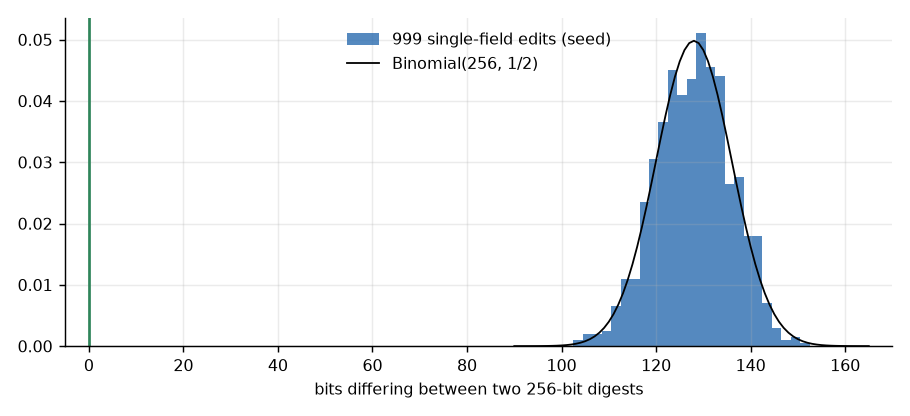
Concept check. Which fields would you add to make A's digest depend on the code it ran? The code version and the image digest, not the tag.
7. Artefacts, roles and the gate
A run is its artefacts plus the manifest that describes them. Each artefact has a role, a format, a required flag and a validation contract. Six roles recur: scalar-summary, trajectory, per-bin-summary, domain-specific, upstream-input, figure. In the toy: trajectory.csv (columns t_s, agent, x_m, required), summary.json (n_agents, mean_speed_m_s, required), per_bin.csv (10 s bins, optional), figure.svg (optional), upstream.json (digest of the input manifest, optional).
A gate refuses a run whose files do not match, at three levels: presence; presence and schema (columns, row count, summary keys); presence, schema and physical bounds. The bound used, 0 \le \bar v \le 3 m/s, is a stated teaching assumption, not a literature value.
In words: the gate is the packing list checked against the box: the right files, the right shape, and numbers a walking person could produce.
Worked numbers (workbook section 7). Gate verdicts by level; "presence", "+ schema", "+ bounds":
| Defect | Presence | + schema | + bounds | Reason |
|---|---|---|---|---|
| none: 5 artefacts, 7212 rows, \bar v = 0.9948 m/s | PASS | PASS | PASS | |
summary.json deleted |
FAIL | FAIL | FAIL | missing required file |
figure.svg deleted (4 artefacts) |
PASS | PASS | PASS | optional file |
x written in centimetres, header still x_m |
PASS | PASS | FAIL | mean speed 99.48 m/s outside 0 to 3 |
| last 10 % of frames dropped | PASS | FAIL | FAIL | 6492 rows, expected 7212 |
A presence-only gate passes the centimetre file. The schema check cannot see the unit because the header is unchanged; only the physical bound does. Week 4 builds on this failure.
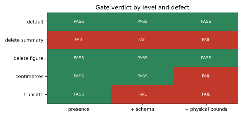
Concept check. Why is a physical bound weaker evidence than a units field in the schema? A bound rejects only values outside a range; a value 100 times too large that still fits the range would pass.
8. Break it: a clock for a seed
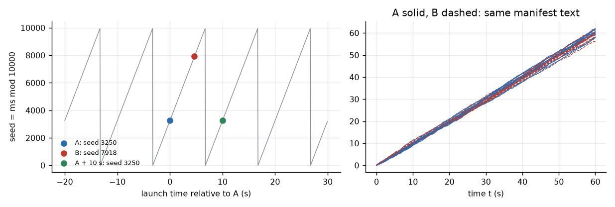
Seeding from the wall clock makes each launch different by accident. With s = (\text{ms since midnight}) \bmod 10000: run A launched at 10:15:03.250 is 36,903,250 ms, seed 3250; run B at 10:15:07.918 is 36,907,918 ms, seed 7918. Two symptoms follow.
- Identical manifests (
seed: "clock", digest startingd1c7f8b7564d) produce different outputs: A gives 60.2669 m (d02b9ddfbf02), B gives 59.6669 m (250df0e7f977). The manifest does not determine the output. - Two launches 10.000 s apart map to the same seed: A + 10 s gives seed 3250 and digest d02b9ddfbf02, byte-identical to A, while being reported as two independent runs. A scripted sweep launching every 10.000 s gives 1 distinct seed in 20 launches.
In words: a clock is a seed nobody chose and nobody wrote down; the packing list says the same thing twice while the boxes hold different things.
Recording the clock-derived seed after launch restores reproducibility (manifest digests af45a2dedaa5 and d4db938cb9f4 now differ, and re-running seed 3250 reproduces A) but not the design: the runs were still not chosen to be independent. For 20 launches at uniformly random instants the chance of at least one seed collision is 1 - \prod_{i=1}^{19}(1 - i/10000) = 0.0188 (the birthday problem, assuming launch instants spread uniformly over the day; one simulated draw of 20 launches had 20 distinct seeds). The corpus is silent on wall-clock seeding hazards; the nearest passage notes that new calculators ship with a factory seed, so two calculators out of the box can produce the same "random" numbers (peck2008_2ba0, Exploration 2.2).
Exam questions
-
State the four inputs of a simulator viewed as a function and give one observation showing that the environment is an input. Model, parameters \theta, seed s, environment e. Switching float64 to float32 in the toy moves the mean final position from 59.6859 m to 59.6856 m and changes the output digest from d489c1ed5e35 to 212ed91b6ca6.
-
Seeds 42 and 43 give sample means of -0.0175 and 0.0125 at n = 1000. Which knob would you turn to make such differences smaller, and by what factor for a tenfold change? The sample count n, not the seed. The spread is \propto 1/\sqrt{n}; n \to 10n shrinks it by \sqrt{10} \approx 3.16. With n from 1000 to 10,000 the sd of 20 means goes from 0.0308 to 0.0098, a factor of 3.1.
-
A generator's histogram is centred at zero with sd 1.109. Can you conclude it is a good generator? What would you check? No. The toy generator (a = 3, m = 31) has mean 0.0226 and sd 1.109 but only 15 distinct values. Check the number of distinct values, the period, and a distributional test such as Kolmogorov-Smirnov (0.1249 for the toy, 0.0269 for the good generator).
-
Two configurations of a simulator are compared, 8 agents against 9. Explain why the comparison is confounded under one shared stream and how per-purpose, per-entity seeds fix it. All later draws shift when a draw is inserted, so every original path changes (8 of 8) and the difference in means mixes the effect of the extra agent with a reshuffle. With a stream per purpose and per agent, keyed by H(s \mid p \mid i), 0 of 8 original paths change. A stream per purpose alone is not enough (8 of 8) when noise is interleaved across agents.
-
A re-run with the seed missing from the manifest gives a mean final position about 0.5 m from the original. Is the re-run faithful? What settles it? Not necessarily. The mean of 60.1893 m differs by 0.5034 m, yet the digest differs, so the re-run is a different run. The digest over the full artefact settles it; a tolerance on one summary number does not.
-
A gate passes a run at "presence only". A trajectory file was written in centimetres. Which checks catch it and why do the others not? Only the physical bound (mean speed 99.48 m/s outside 0 to 3 m/s). Presence sees the file; the schema sees the right columns and the right row count (7212) because the header still reads
x_m.
Further reading
- SIM507 Curriculum for the course arc.
- kroese2019_3738: recurrence (eq. 3.1), Box-Muller (Algorithm 3.2.1), Monte Carlo interval (eq. 3.13), common random numbers (Chapter 3 exercises).
- wasserman2004_ea08 ↗: Example 24.1.
- guarino2026_e72c ↗: dependency grading and reproducibility criteria for CSI sensing.
- kleinmeier2019_e6cd ↗: commit hash in output, JSON inputs.
- dhillon2017_6a80 ↗: definition of a one-way hash.
- peck2008_2ba0: pseudo-random numbers and the factory seed shared by new calculators.
- pride2025_51f1 ↗: secondary report of the failed-reproduction survey, and the case for archiving code, parameters, dependencies and environment.
Corpus gaps, stated once: the corpus is silent on the minimal standard generator's constants and its small-seed weakness, on hash-derived substreams, on wall-clock seeding hazards, on content-addressed storage and canonical serialisation, on manifests for containerised simulation workflows, and on floating-point determinism across numeric environments.
Provenance (instructor only)
obsidian/monad-knowledge/edu/courses/SIM507-simulation-toolkits/SIM507 Curriculum.md(course note)
This week quotes no first-party measurement. All numbers are closed forms, literature values, or outputs of workbook.ipynb (also in numbers.json).