Reader companion to the slide deck. It follows the deck section by section. Each section has the idea, the derivation with an "In words:" gloss, the worked numbers, and one concept check. Every number is printed by workbook.ipynb (numpy, scipy, matplotlib only) and collected in numbers.json. Numbers labelled simulated come from the workbook's two-chain toy channel with a seeded generator; numbers labelled measured come from first-party hardware and are introduced with their setup. A widget in the deck at its default state shows the same number as the workbook.
Conventions. The grid is the 56-tone HT20 grid, tones k=-28..-1, 1..28, spacing \Delta f = 312.5 kHz. "One tone" means k=+10. A packet stream is 600 packets at 100 packets per second, with one moving path modulated at 0.9 Hz. The generator is a 32-bit linear congruential generator with Box-Muller normals; the exact recipe is in the first cell of the workbook.
1. The measurement model
What a commodity card reports for receive chain r, tone k, packet t is well described by
In words: the reported number is the physical channel, multiplied by one real gain and one phase ramp that the receiver invents per packet, plus noise.
- H_r(k,t) is the physical channel, the multipath sum of W1 and W2. It is the only term that describes the room.
- g(t) is the automatic gain control (AGC) gain. A front end must span tens of dB between a near and a far transmitter, and a 10-bit converter spans about 60 dB, so the loop rescales every packet before the FFT. The gain is common to all tones and is not reported.
- \phi(t) is the per-packet phase intercept. Two crystals disagree by parts per million, and the receiver corrects the carrier offset from the preamble only approximately. The standard allows the carrier to drift by up to 100 kHz at 5 GHz, and at 4000 frames per second that can move the phase by up to 50\pi between consecutive CSI values (wang2015_48cf ↗). The packet-boundary detector adds a second contribution, because it lands on a slightly different sample each time (xie2015_0389 ↗).
- \beta(t)\,k is the timing slope. A timing error \tau multiplies tone k by e^{-j2\pi k\Delta f\tau} (shift theorem), so \beta=-2\pi\Delta f\,\tau. One sample of error at 20 MHz is \tau=50 ns, which gives \beta = 0.0982 rad per tone and a tilt of 5.50 rad across 56 tones.
- n_r(k,t) is thermal noise, the only term that behaves as in the textbooks.
Two properties drive the week. The three receiver terms are time-varying and unobserved, so no offline calibration removes them (ma2020_4782 ↗). And g, \phi, \beta carry no chain index r: the chains of one receiver share the oscillator, the sampling clock and, to first order, the gain step.
Worked numbers (simulated, defaults: gain spread 3 dB, intercept std 3.5 rad, slope std 0.05 rad per tone, noise 0.10). Packet 0 at tone 10 has gain -0.70 dB, intercept 0.445 rad and slope 0.0124 rad per tone, so the receiver adds 0.445+10\cdot0.0124=0.569 rad. The channel amplitude and phase are 1.539 and 0.198 rad; the reported values are 1.324 and 0.756 rad, the difference being the noise term. Over 600 packets the circular standard deviation of the reported phase at tone 10 is 2.565 rad with all terms on, 0.537 rad with the intercept off (the slope alone contributes about 10\cdot0.05 rad), 0.119 rad with only gain and noise on, and 0.108 rad with the channel alone (the motion). The amplitude at tone 10 varies with a standard deviation of 3.18 dB with the gain on and 1.31 dB with it off.
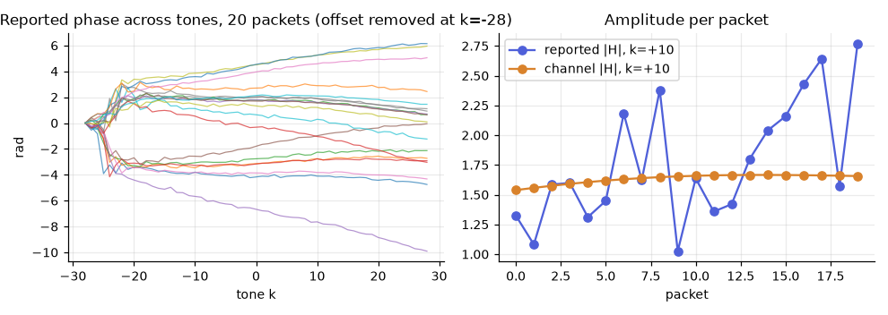
Concept check. Which of the three receiver terms would you expect to leak a small chain dependence in real hardware? (Answer: the gain, because each chain has its own analogue amplifier stages; the ratio therefore carries a per-device constant, section 5.)
2. How bad is a random phase
Phase lives on a circle, so dispersion needs its own estimator. Map each phase to a unit phasor, average, and take the length of the average:
In words: if all phases agree the phasors add up and \bar R\to1; if they are spread around the circle they cancel and \bar R\to0, and \sigma_c grows without bound.
For a wrapped normal with parameter \sigma the expected \bar R is e^{-\sigma^2/2}, so \sigma_c=\sigma. A finite sample of uniform phases never gives \bar R=0: the phasors form a random walk and \bar R is of order 1/\sqrt N. That puts a ceiling on the estimate, \sigma_c\approx\sqrt{-2\ln(1/\sqrt N)}=\sqrt{\ln N}.
Worked numbers (simulated, seed 502). The ceiling is 1.517 rad at N=10, 2.146 rad at N=100, 2.529 rad at N=600 and 2.628 rad at N=1000. For the wrapped normal with \sigma=3.5 rad the theoretical \bar R is 0.00219, twenty times below the noise floor 1/\sqrt{600}=0.0408; the sample gives \bar R=0.0275 and \sigma_c=2.681 rad. A uniform sample of 600 gives \bar R=0.019 and \sigma_c=2.815 rad; a uniform sample of 100 gives 0.125 and 2.038 rad. The ceiling is a typical value, not a bound: one draw lands on either side of it. To see \sigma=3.5 rad through the noise floor one would need N=e^{3.5^2}\approx2.1\times10^5 packets. For small spreads the estimator is honest: true 0.3, 1.0, 2.0 rad read 0.305, 1.007, 1.952 rad at N=600.
Reading rule: a circular standard deviation pinned near \sqrt{\ln N} means "indistinguishable from uniform", not "2.5 rad of spread".
Concept check. A colleague averages the raw phase over 100 packets to beat the noise down. What does the mean phasor look like? (Answer: its length is a random \sim0.1; here 0.125. The result estimates the mean of a random draw, not the channel.)
3. The two-chain ratio
Both chains of one receiver see the same corruption, so divide:
In words: whatever value the gain, the intercept and the slope took on this packet, they appear once above and once below and vanish. Nothing is estimated, so nothing is fitted away (zeng2021_1e4f ↗; wu2022_75d3 ↗). Noise is the exception: it is added after the gain and is not common, which is why the result is cleaner but not perfect.
What survives is the ratio of two physical channels seen from antennas a few centimetres apart. If one path moves and the rest are static, H_i = H_{s,i} + A_i e^{-j\theta_i(t)}. For antennas a few centimetres apart the difference \theta_2-\theta_1 of the reflected path lengths is nearly constant over a short movement, so the ratio depends on one unit phasor Z=e^{-j\theta_1(t)} and is a Möbius transformation of it (zeng2021_1e4f ↗). Möbius maps send circles to circles, so the motion signature survives the division.
The classical alternative for one chain is the linear fit across tones, subtracting \phi+\beta k per packet (ma2020_4782 ↗). It works, but it removes any true delay (section 10).
Worked numbers (simulated, seed 503). At tone 10 the raw phase of chain 1 has \sigma_c=2.600 rad and chain 2 has 2.617 rad (the realised intercept std is 3.517 rad). The ratio phase has \sigma_c=0.129 rad, a factor 20.1 lower. Of that 0.129 rad, the true H_1/H_2 phase itself swings with \sigma_c=0.095 rad (the motion), and the error against that truth is 0.086 rad. With the noise switched off the ratio equals H_1/H_2 to 1.4\times10^{-15}. The spectrum of the ratio phase peaks at 0.891 Hz (motion at 0.9 Hz) and holds 0.259 of its power within 0.8 to 1.0 Hz; the raw phase peaks at 0.183 Hz, meaningless, with a share of 0.068. Away from the defaults: with the intercept off the raw phase tightens to 0.498 rad (the slope term alone) while the ratio stays at 0.128 rad, so the reduction falls to 3.9; with noise 0.30 the ratio widens to 0.289 rad (error against truth 0.272 rad) while the raw phase stays near uniform (2.645 rad); with slope std 0.2 rad per tone the ratio is 0.126 rad; with motion at 1.5 Hz or 0.2 Hz the ratio-phase peak moves to 1.514 Hz or 0.293 Hz while the raw peak stays at 0.171 Hz.
Measured. On a link between an AX210 transmitter and an AX210 receiver with two active antennas, in an office, the raw per-packet phase intercept had a standard deviation of 3.5 rad. On a 30-minute daytime baseline of the same kind of link, the ratio phase had a circular standard deviation of 0.26 rad. The simulated value (0.129 rad) is smaller. The simulated noise level of 0.10 is a round default, not a fit, so the comparison supports the direction and the mechanism, not the last digit.
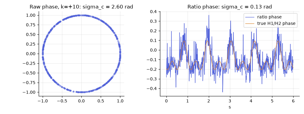
Requirement. The ratio needs two active receive chains in every record. A capture with one chain, or one that silently drops to one, cannot be repaired afterwards, because the simultaneous second view under the same oscillator was never recorded.
Concept check. Why can the ratio not be applied to the two receive chains of two different cards? (Answer: separate oscillators, so the corruption is no longer common and does not cancel.)
4. Division or conjugate multiplication
The conjugate product \hat H_1\overline{\hat H_2} has phase \arg H_1-\arg H_2: the common phase cancels by subtraction. The gains multiply, g^2|H_1||H_2|, so the product repairs phase but squares the amplitude problem. The ratio has amplitude |H_1|/|H_2| and cancels the gain, but its denominator can fade.
In words: division is exact until the denominator chain fades into the noise; the product never blows up but it is not gain-free.
Worked numbers (simulated, seed 504; chain 2 fades by the stated depth around t=3 s, noise floor 0.10 added afterwards). The phases of the two outputs are identical (the same \arg), with error against the noise-free truth inside the fade of 0.090, 0.410, 0.602 and 0.728 rad at depths 0, 20, 30 and 40 dB. The amplitudes differ. Fitting \ln|Q| on \ln g gives a slope of -0.009 for the ratio and 1.989 for the product. Variance of the tone-10 amplitude, normalised by its squared median:
| fade depth (dB) | ratio | product |
|---|---|---|
| 0 | 0.0499 | 0.942 |
| 20 | 2.095 | 1.307 |
| 30 | 6.841 | 1.350 |
| 40 | 21.05 | 1.375 |
The largest ratio amplitude grows from 1.85 to 19.79, 32.55 and 101.2, while the largest product amplitude stays at 14.75, set by the gain excursions and bounded by |\hat H_1||\hat H_2|. Neither is free: the product carries g^2 (0.942 at depth 0 against 0.050), the ratio carries the fade.
Hardware note. On one AX210 capture the conjugate product of the two chains had a standard deviation of 2.2 degrees around two discrete states. The mechanism is not established in the sources read for this course.
Concept check. Which output would you pick for a Doppler spectrum of amplitude, and which for a phase-only feature? (Answer: the ratio for amplitude when the denominator is healthy, either for phase because the phases are identical.)
5. The AGC diary
The reported amplitude is |\hat H_r|=g\,|H_r|. The tempting per-packet feature, the mean level across tones,
is proportional to g(t) when the room is quasi-static: the feature is the gain. In words: a per-packet gain moves every tone together, so it can forge absolute levels but not the shape across tones or the dynamics across packets, and the ratio removes it outright.
Worked numbers (simulated, seed 505, gain spread 3 dB). The per-tone amplitude CV (standard deviation over time divided by the mean, averaged over tones) is 0.4265 raw and 0.2548 for the ratio, a factor 1.67. The correlation between the per-packet mean amplitude and the hidden gain is 0.9988 raw and -0.169 for the ratio; the ratio is not exactly zero because the noise is added after the gain and is not common. The CV of a lognormal gain alone with 3 dB spread would be 0.356. The ratio does not always win: with no gain spread the CV is 0.214 raw and 0.231 for the ratio (a ratio of two noisy numbers is noisier); with 6 dB spread it is 0.801 raw and 0.318 for the ratio. If chain 2 sits 7 dB lower than chain 1, the ratio level shifts by 6.97 dB and its CV rises to 0.314, because the weaker chain has a lower signal-to-noise ratio.
Measured (the office baseline of section 3). Per-tone amplitude CV was 0.32 raw and 0.20 for the ratio. The two chains of one receiver can differ in RSSI by up to about 7 dB, so the ratio carries a per-device constant; compare shapes and changes, not absolute ratio levels across devices.
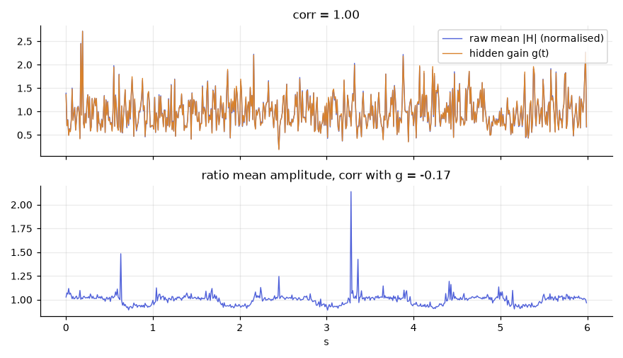
Concept check. Which of these survive the AGC: (a) mean |\hat H| across tones; (b) the tone vector divided by its own mean; (c) the variance over time of (a); (d) the frequency of the dominant spectral peak of the ratio amplitude? (Answer: (b) and (d); (a) and (c) read the gain.)
6. Lose a chain
A record whose second chain is reported at RSSI -127 ("no measurement") carries a stale duplicate block for that chain. The sources read for this course do not say what the block duplicates, so the workbook models two hypotheses: (a) a copy of the last good chain-B block, (b) a copy of the chain-A block of the same record.
Worked numbers (simulated, seed 506, 20 % stale records requested). 130 of 600 records are stale (usable fraction 0.783). On the usable records the ratio phase has \sigma_c=0.121 rad. Over all records under hypothesis (a) it is 0.735 rad, because each stale record divides by an old block with a different random intercept. Under hypothesis (b) the stale ratio is exactly 1 (deviation 10^{-16}) and the all-record value is 0.116 rad, indistinguishable from a healthy stream. With every record stale: 2.919 rad under (a); 0.009 rad under (b), a perfectly constant series that reads as a still room. With chain B absent the usable fraction is zero.
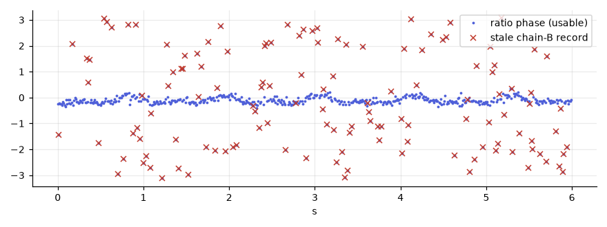
Rule: filter on the per-chain RSSI flag before dividing, and treat a stream whose ratio is suspiciously constant as a capture defect until proven otherwise. No later algorithm recovers a one-chain capture.
Concept check. Why does a constant ratio series not prove an empty room? (Answer: a stale block copied from the other chain gives exactly 1, and no motion, whatever the room does.)
7. Divide the right things
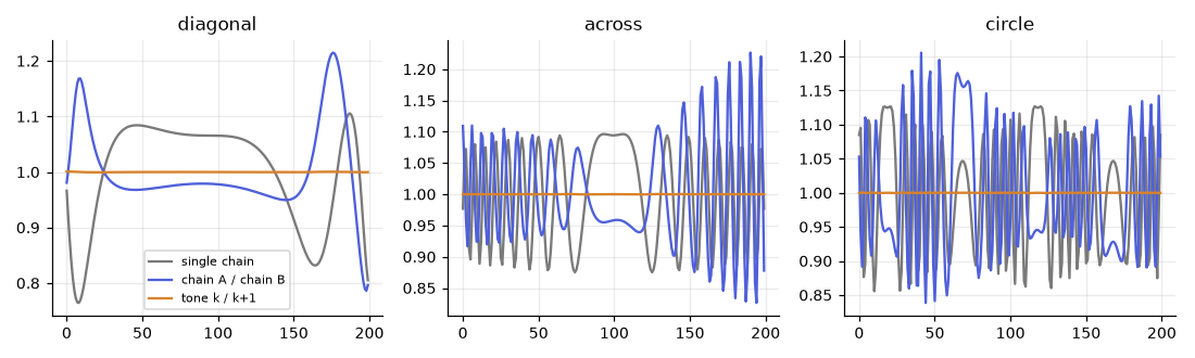
Dividing tone k by tone k+1 of one chain also cancels the AGC gain, since the gain is common to all tones. But the physical content is different. A walker's contribution across neighbouring tones differs only by e^{-j2\pi\Delta f\tau}, where \tau is the path delay: 0.0393 rad for \tau=20 ns and 0.0982 rad for 50 ns. Neighbouring tones 312.5 kHz apart see nearly the same channel, so their ratio is a local spectral slope, not a spatial ratio, and keeps almost none of the walker's signal.
A processing chain of ours once computed exactly this quantity while calling it the two-chain ratio: the storage was chain-major (all tones of chain 1, then chain 2) and the reader assumed tone-major, so each "ratio" divided adjacent tones of one chain. Amplitude-only unit tests passed, because the wrong quantity is still gain-free. The remedy is a test that pins the reshape against the reader on real data.
Worked numbers (simulated). A toy room of 4 by 3 m at 5.2 GHz (wavelength 5.77 cm), transmitter at (0.5, 0.5), receiver chains 3 cm apart, line of sight plus four wall images (reflection 0.6), one walker as a point scatterer. Signal metric: median over tones of the RMS deviation of the series from its mean, relative to the mean; "kept" is the metric of the quantity divided by that of a single chain.
| walker path | single-chain metric | chain A / chain B kept | tone k / k{+}1 kept |
|---|---|---|---|
| diagonal | 0.1247 | 0.837 | 0.326 % |
| across | 0.1042 | 1.108 | 0.249 % |
| circle | 0.1134 | 1.074 | 0.243 % |
An earlier analysis of a different toy two-antenna model (a 4 by 3 m room as well) reports 0.4 to 1.9 % for the adjacent-tone quantity and 0.93 to 1.65 for the two-chain ratio. The ranges differ because the models differ; the conclusion is the same: percent versus order one.
Concept check. A series is AGC-free. Does that make it a two-chain ratio? (Answer: no; AGC-freedom is necessary, not sufficient. Check which two things were divided.)
8. Window, then threshold
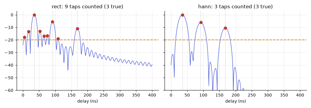
On an N-tone grid the delay resolution is 1/(N\Delta f): 12.5 ns per bin for 256 tones (80 MHz) and 50 ns for 64 tones (20 MHz). No path lands on the grid. The implicit rectangular window has a Dirichlet transform whose first sidelobe is at -13.26 dB, so an off-grid tap leaks ghosts that look like multipath. A Hann window lowers the first sidelobe to -31.47 dB and widens the main lobe (the full -3 dB width goes from 0.886 to 1.446 bins, the first null from 1.00 to 2.01 bins). A tap threshold, for example -20 dB below the strongest peak, is meaningful only after the window.
Worked numbers (simulated). Three taps at 35, 92 and 168 ns with amplitudes 1.0, 0.5 and 0.3, zero-padded 16-fold; census = interior local maxima at or above the threshold.
| bandwidth, window | -10 dB | -20 dB | -30 dB | -40 dB |
|---|---|---|---|---|
| 80 MHz, rectangular | 2 | 9 | 16 | 29 |
| 80 MHz, Hann | 2 | 3 | 4 | 6 |
| 20 MHz, rectangular | 1 | 3 | 5 | 5 |
| 20 MHz, Hann | 1 | 1 | 1 | 1 |
At 80 MHz with the rectangular window and -20 dB the census is 9: the three true taps plus six ghosts between -13 and -19 dB; with Hann it is exactly the three true taps (at 35.2, 92.2 and 168.0 ns, 0, -6.0 and -10.4 dB). At -10 dB even Hann counts two, because the third tap sits at 20\log_{10}0.3=-10.46 dB (read at -10.44 dB with Hann, -10.94 dB with the rectangular window). A higher threshold is not a repair: with the rectangular window a -12 dB threshold happens to count 3, because the strongest ghost (-13.3 dB) is 2.4 dB below the third tap, but lower that tap to 0.1 (true level -20 dB, read at -20.57 dB) and it is weaker than all six ghosts (-19.0 to -12.9 dB), so no threshold keeps it and drops them. With Hann the same weak tap is a clean peak at -19.98 dB (census 3 at -20 dB; 4 at -30 dB, the extra one a ghost at -29.2 dB). At 20 MHz the rectangular count of 3 is a coincidence: the peaks are at 37.5, 184.4 and 250 ns, the 92 ns tap is missing and 250 ns is a ghost. Hann at 20 MHz returns one merged peak at 46.9 ns: taps 57 and 76 ns apart are inside the widened main lobe. Windowing trades resolution for cleanliness; bandwidth sets the resolution.
Delay profiles on commodity cards need the phase-error compensation first, delay-domain reading second (xie2015_0389 ↗).
Concept check. A pipeline reports 9 taps above -20 dB on a channel known to have 3. Why does raising the threshold not fix it cleanly? (Answer: the ghosts reach -13.3 dB, so a threshold works only when every true tap is stronger than the strongest ghost. Here -12 dB works with 2.4 dB of margin; a true path at -20 dB is lost at any threshold. Window first.)
9. Scope every statistic
A passive capture on a live channel interleaves whatever the air produces: different record classes (tone count, modulation) from different transmitters at different power. Pooling them makes every statistic a mixture artefact.
Worked numbers (simulated, seed 509, 2000 records, 74 % legacy 52-tone drawn, realised 0.7425; sources 12 dB apart, 2 dB spread each). Legacy records have no tones at |k|=27,28, so zero-padding to the 56-tone grid fakes a band edge. The per-tone CV at the padded tones is 1.744 pooled; a Bernoulli mixture of zero and a constant predicts \sqrt{0.7425/0.2575}=1.698. Scoped to HT-56 the same tones give 0.201. The interior CV is 0.198 pooled and 0.199 scoped, so the artefact sits at the edge only; the pooled mean amplitude at the edge tones is 0.185 of the interior against 0.708 scoped. The pooled RSSI has a standard deviation of 5.57 dB against 1.98 dB (legacy) and 1.92 dB (HT-56); with no offset it is 1.96 dB, with a 6 dB offset 3.25 dB. With a 50/50 mix the edge CV falls to 1.07 and the RSSI spread rises to 6.29 dB.
Measured. A 2.4 GHz channel-11 ambient capture was 74 % legacy-52 records and 26 % HT-56 records.
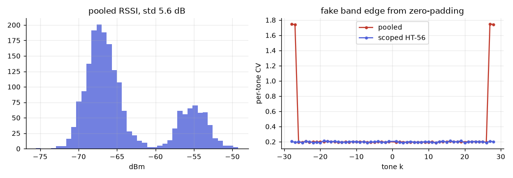
Rule: scope every statistic to one (tone count, modulation) record class and one source before computing anything. It costs one groupby.
Concept check. A pooled capture shows an RSSI spread of 6 dB and a huge CV at the last four tones. Two explanations? (Answer: a wildly dynamic channel with band-edge fading, or a mixture of two transmitters and a zero-padded class. Group by class and source first.)
10. The linear phase fit and what it removes
Fitting \phi+\beta k across tones by least squares and subtracting it stabilises the phase. But a pure delay is also linear in k, with slope -2\pi\Delta f\tau. The fit removes the geometry along with the corruption, so absolute time of flight is lost; curvature (multipath structure) and change over time remain.
Worked numbers (simulated). Planted delay 20 ns (a path length of 5.996 m), common offset 1.0 rad, slope 0.05 rad per tone, plus a nonlinear ripple 0.35\sin(k/9). The planted delay slope alone would be -0.0393 rad per tone. The measured phase, unwrapped, has a fitted slope of +0.0223 rad per tone, so the delay read from it is -11.35 ns. With no timing slope it would read 14.12 ns (the ripple contributes a bias). After subtracting the fit the residual standard deviation is 0.1585 rad and the recovered delay is 0 by construction. In the default view the phase has 0 wrap jumps and an unwrapped span of 1.03 rad.
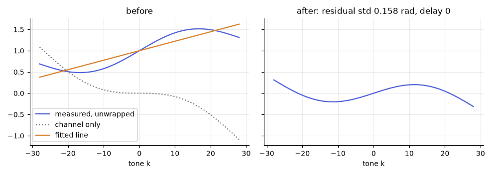
Concept check. Why is the delay read before the fit not the planted delay? (Answer: the receiver's timing slope adds to it and cannot be told apart; only a cross-chain quantity such as the ratio removes the receiver's part without removing yours.)
Step zero and hand-off
Verify the parse first. Reading the imaginary word first maps H\mapsto j\overline H: the amplitude is unchanged (maximum difference 0.0 in the workbook) but the phase is mirrored and the delay profile is time-reversed, so a causal channel becomes anti-causal. The early-to-late energy ratio of the Hann-windowed profile separates them: 4722 for the correct parse and 0.0076 for the swapped parse in a noise-limited simulation. Measured on a real AX210 capture that had first been read in the wrong order: an early-to-late tap ratio of 21.3 for the correct parse and 0.48 for the swapped. The source does not record the exact windows of that ratio, so compare the side of 1, not the value with the simulation. A ratio below 1 is a wrong parse, not a strange room.
Hand-off to the lab and to W6. A sanitised ratio series (seed 5100, 600 packets, 56 tones) has \sigma_c=0.123 rad at tone 10, a temporal standard deviation of the unwrapped ratio phase of 0.123 rad, a peak at 0.903 Hz, a correlation with the hidden gain of -0.167, and a spread of 0.220 across tones of its per-tone mean amplitude. What survives is relative (across tones) and temporal (across packets). Absolute delay and absolute level do not.
Exam questions
Q1. The cancellation. Starting from the measurement model, derive the two-chain ratio and state the physical assumption behind the cancellation. Why can a one-chain capture not be repaired afterwards? Model answer. Division removes g and e^{j(\phi+\beta k)} because neither carries a chain index, giving H_1/H_2. The assumption is that both chains share the oscillator, the sampling clock and the gain step. A one-chain capture never recorded the simultaneous second view under the same oscillator state, so the information needed for the cancellation is not in the file.
Q2. A saturated estimator. A student reports "circular std 2.4 rad over 600 packets, so the corruption is smaller than the 3.5 rad measured". Correct them. Model answer. For near-uniform phase \bar R is of order 1/\sqrt N\approx0.04, so \sigma_c\approx\sqrt{\ln 600}=2.53 rad is the estimator ceiling, not a spread. Any dispersion near or above a full turn gives the same reading. 2.4 and 3.5 are not comparable; the phase is indistinguishable from uniform.
Q3. Feature autopsy. For each feature say whether it survives AGC: (a) per-packet mean amplitude across tones; (b) tone vector divided by its own mean; (c) the variance over time of (a); (d) the dominant spectral peak of the ratio amplitude at one tone. Model answer. (a) dies, proportional to g (correlation 0.9988 in the workbook). (b) survives, g cancels. (c) dies, it is the variance of the gain. (d) survives, the ratio removed the common gain and a spectral location is invariant to residual scale.
Q4. The census that lied. A pipeline reports 9 taps above -20 dB on a channel with 3. Diagnose and explain why a higher threshold is the wrong repair. Model answer. No window before the IFFT: off-grid taps leak sidelobes at -13.3 dB that clear the threshold. Hann lowers them to -31.5 dB and the census returns 3. A higher threshold works only while every true tap is stronger than the strongest ghost: here -12 dB happens to count 3, with 2.4 dB of margin, and a true path weaker than the ghosts (one at -20 dB) is lost whatever the threshold. The cost of Hann is resolution: at 20 MHz taps 57 and 76 ns apart merge.
Q5. The wrong ratio. A colleague's "ratio" is AGC-free and looks like a motion detector, but it responds to a walker with 0.3 % of the strength of a single chain. What did they compute, and how do you check? Model answer. Probably the ratio of neighbouring tones of one chain: a gain-free spectral slope. Neighbouring tones differ by e^{-j2\pi\Delta f\tau}, only 0.04 to 0.10 rad for 20 to 50 ns delays. Check by comparing the code's reshape against the reader on a real record, and test the quantity against the two-chain ratio on the same data.
Q6. The pooled capture. An ambient capture gives an RSSI spread of 6.5 dB and a CV of 1.7 at the last four tones. Offer an alternative to "very dynamic channel with band-edge fading" and the remedy. Model answer. A mixture of two record classes from two sources at different power: bimodal RSSI (per-source spreads about 2 dB) and a zero-padding artefact at the edge tones (scoped CV about 0.2). Group by (tone count, modulation) and source before any statistic.
Further reading
- zeng2021_1e4f ↗: the ratio as an observable, with the noise-cancellation argument and the antenna-pair views.
- wu2022_75d3 ↗: the Fresnel-zone model extended to the ratio, and why raw phases of two antennas jump randomly while the ratio does not.
- ma2020_4782 ↗: survey treatment of phase offsets and the linear-fit removal.
- wang2015_48cf ↗: why raw CFR phase is unusable on commodity cards, and the CFO magnitude argument.
- xie2015_0389 ↗: packet-boundary and CFO error sources, and the sanitisation that precedes a delay profile.
- zheng2019_5389 ↗: a feature built entirely from sanitised, relative and temporal structure.
- gringoli2019_68e7 ↗: the firmware-level CSI extractor that made cross-checking extracted CSI practical.
Provenance (instructor only)
Not for slides or students. First-party numbers and where they come from:
obsidian/monad-knowledge/_knowledge/methods/csi-drift-estimation.md: CV 0.32 raw and 0.20 for the ratio; ratio phase circular standard deviation 0.26 rad (30-minute daytime baseline, AX210 path). The note does not name the room or say which reader computed the ratio; "office" and the transmitter-receiver pairing come from the previous revision of this lecture (below). Whether that baseline predates the storage-layout defect of section 7 is not established in the sources read.obsidian/monad-knowledge/diary/2026-09-23 - The lake's ratio columns divide neighbouring tones of one chain, not chain A by chain B.md: adjacent-tone quantity keeps 0.4 to 1.9 % of a walker's single-chain signal, the two-chain ratio 0.93 to 1.65 (4 by 3 m toy model); the storage-layout defect in section 7. Caution recorded there: lake-derived "ratio" statistics from before 2026-09-23 (for example 0.034 dB within a session) are the adjacent-tone quantity and are not evidence that AGC is common to both chains..claude/memory/csid-capture-service.md: two active chains as a hard requirement; RSSI -127 chain block is a stale duplicate; conjugate product 2.2 degrees around two discrete states (mechanism not established); early/late tap ratio 0.48 swapped against 21.3 correct (window definition not recorded).- Literature passages read for this revision (search_vault): the 100 kHz / 4000 frames per second / 50\pi figure in wang2015_48cf; the constant path-length difference behind the Möbius form in zeng2021_1e4f and wu2022_75d3.
.claude/memory/lake-findings-2026-08.md: per-node chain RSSI offset up to +7 dB (an RSSI field, unaffected by the layout defect).- Previous revision of this lecture (
obsidian/monad-knowledge/edu/courses/WS501-wifi-csi-sensing/week-05-preprocessing/lecture.md, git history before 2026-09-28): raw per-packet phase intercept std 3.5 rad; the 2.4 GHz channel-11 ambient mix of 74 % legacy-52 and 26 % HT-56. Copied from that text; not re-derived from the archive in this rebuild. - Literature, resolved by key with
cite_resolve:literature/Boosting WiFi Sensing Performance via CSI Ratio.md,literature/WiFi CSI-based device-free sensing from Fresnel zone model to CSI-ratio model.md,literature/WiFi Sensing with Channel State Information.md,literature/Understanding and Modeling of WiFi Signal Based Human Activity Recognition.md,literature/Precise Power Delay Profiling with Commodity WiFi.md,literature/Zero-Effort Cross-Domain Gesture Recognition with Wi-Fi.md,literature/Free Your CSI.md. - Textbook constants recomputed in the workbook: rectangular first sidelobe -13.26 dB, Hann -31.47 dB, full -3 dB widths 0.886 and 1.446 bins, 12.5 ns per bin at 80 MHz.
- Every simulated number, including the widget states away from the defaults, is printed by
workbook.ipynb(section 5.13 for the sweeps) and stored innumbers.json.