Companion to the interactive deck. The deck is primary; each widget in it has a section here with the derivation, the worked numbers and one concept check. Every number below is printed by workbook.ipynb (same seeds, same formulas as the widgets at their default state) and stored in numbers.json. Numbers labelled "measured" come from a first-party rig and are introduced together with their setup.
Where this week sits. Week 1 gave the echo rotation f_D = 2v/\lambda. Week 3 gave the record clock: what one CSI record is and when the card stamps it. This week asks what sets the spacing of those records in time, how to tell a delivered record from a commanded one, and how the standard changes who sends the sounding frames. Week 5 assumes a stream whose timing is known and scoped to one transmitter.
1. Who sends the frames you measure
CSI exists only when a frame arrives. Three ways to get frames:
- Ambient listening. Measure whatever the air carries. The arrival process is set by other people's traffic: bursty, load-dependent, different every hour.
- Paced injection. Transmit your own frames on a fixed slot grid T = 1/R. The rig used here is an AX210 in monitor mode injecting legacy OFDM frames of 200 bytes at 6 Mb/s, 25 to 250 per second. Injection is used because the card cannot act as an access point. On 2.4 GHz the driver falls back to 1 Mb/s DSSS for group-addressed frames unless the OFDM rate is forced, and DSSS frames carry no CSI. Pacing uses absolute deadlines: a missed slot is skipped, never bunched into the next one.
- 802.11bf session. The sensing initiator schedules the sounding frames itself (sections 7 and 8).
Two numbers describe how well a paced stream did:
In words: delivered rate counts frames that reached the receiver; occupancy counts how many grid slots got one. A frame deferred out of its own slot is delivered but leaves its slot empty, so the two differ.
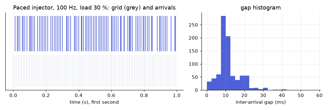
Model used in the widget (a mechanism sketch, not a fit). Each slot is dead with probability 0.5L (never sent); otherwise the frame leaves at the slot start, or with probability L (busy channel) after an exponential deferral of mean 0.6\,T. L is the channel load.
Worked numbers (10 s window, R = 100 Hz, L = 30\%, seed 7):
| Stream | Delivered (Hz) | Occupancy | Gap CV |
|---|---|---|---|
| Paced injector | 86.3 | 0.828 | 0.503 |
| Ambient bursty, nominal 100 Hz | 82.9 | 0.262 | 2.153 |
| Both (paced plus ambient at nominal R L) | 106.2 | 0.846 | 0.687 |
The paced stream sits near its commanded rate but is not on the grid: 863 frames arrive in 10 s while 82.8 slots per second are occupied. The ambient stream delivers a similar count with a quarter of the slots occupied and a gap CV above 2. (Its rate is nominal: bursts start at R/(1+8L) per second and hold 1 + \lfloor \mathrm{Exp}(8L) \rfloor frames, whose mean is below 1 + 8L, so the realised rate is 82.9 Hz, not 100 Hz.) Load ladder for the paced stream: at 0 % the stream is exact (100 Hz, occupancy 1.0, CV 0.0); at 60 % it delivers 72.1 Hz (occupancy 0.676, CV 0.656); at 90 % it delivers 57.0 Hz (occupancy 0.525, CV 0.768).
Measured. One injector and one receiver, slot 10 ms (commanded 100 Hz), one channel per band, the two runs 39 minutes apart. On a 5 GHz channel (channel 36) the receiver got 99.4 of 100 Hz (gap CV 0.083, pooled over all transmitters heard). On a 2.4 GHz channel (channel 6) it got 61.3 of 100 Hz (pooled CV 0.714). The 38.7 Hz deficit has two causes. About two thirds (25.5 Hz) are dead slots: the frame was never transmitted. The remaining 13.2 Hz are frames delayed by CSMA/CA, so they arrive off the grid. Coefficient of variation cannot separate these; slot occupancy and the distribution of consecutive-miss run lengths can. One caveat travels with these numbers: the 5 GHz capture held 12 transmitters, so a timing statistic is meaningful only after scoping to one (section 5).
Concept check. A capture shows 61 Hz delivered against 100 Hz commanded. Which statistic separates dead slots from deferral? Answer: slot occupancy (dead slots leave slots empty and stay empty; deferred frames show up as a frame in a neighbouring slot) together with the miss-run length distribution. The CV of the gaps mixes both.
2. Packet rate is a speed limit
A reflector moving at radial speed v makes the echo phasor rotate at
Packets sample that rotation at rate PRR. Between two packets the phasor advances \Delta\varphi = 2\pi f_D/\text{PRR}. A phase step can be told apart from its negative only if |\Delta\varphi| < \pi, so |f_D| < \text{PRR}/2 (Nyquist), and with f_D = 2v/\lambda:
In words: the echo arrow turns twice per wavelength of walking, and the packets must catch it at least twice per turn. The factor 4 is 2 from the round trip and 2 from Nyquist.
The same bound is written for radar as V_\text{max} = \lambda/(4T_c) with chirp period T_c (soumya2023_9b9f ↗), and as v_\text{max} = \lambda/(4\,\text{PRI}) for 802.11bf passive sensing in the 60 GHz band (ropitault2024_db32 ↗). The packet rate plays the role of the pulse repetition frequency. An ISAC survey, summarising an 802.11p OFDM radar study, states the same dependence qualitatively: velocity ambiguity is inversely proportional to the carrier frequency and to the detection sampling interval (wang2022_2397 ↗).
Beyond the limit the line folds:
Worked numbers (v = 1.0 m/s, 5.2 GHz, \lambda = 5.765 cm):
- f_D = 34.69 Hz. At PRR = 100 Hz, v_\text{max} = 1.441 m/s, the phase step is 124.9 degrees, the line is resolved, and the minimum rate is 4v/\lambda = 69.4 Hz.
- v_\text{max} at 20, 40, 100, 250 and 1000 Hz: 0.288, 0.577, 1.441, 3.603 and 14.413 m/s.
- At PRR = 40 Hz the phase step is 312.2 degrees, and f_\text{alias} = -5.31 Hz. The walker reads as a drift of -0.153 m/s: slow and moving the wrong way. A zero-padded FFT of the sampled phasor peaks at -5.31 Hz, matching the formula. At 20 Hz the alias is also -5.31 Hz (34.69 differs from -5.31 by exactly 40 Hz, which is a multiple of 20).
- Without I/Q (magnitude only) the spectrum is symmetric and the sign is lost: the walker reads as 5.31 Hz of unknown direction.
- Near the ceiling the failure is quiet. At 1.5 m/s the Doppler is 52.04 Hz, above the 50 Hz limit for 100 Hz packets; it folds to -47.96 Hz, which reads as a walker at 1.383 m/s going the other way.
- Band changes the ceiling. At 100 Hz, v_\text{max} is 3.075 m/s at 2.437 GHz, 1.441 m/s at 5.2 GHz and 1.254 m/s at 5.975 GHz; the Doppler of a 1 m/s walker is 16.26, 34.69 and 39.86 Hz.
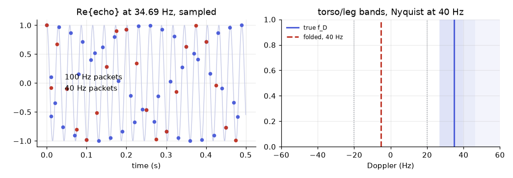
What walking needs. A gait study measured torso Doppler of 27 to 46 Hz and swinging-leg Doppler of 40 to 60 Hz on a 5 GHz link, with f = 2v/\lambda and \lambda = 5.79 cm, so 1 m/s gives 34.54 Hz (wang2016_6482 ↗). Computed here with v = f\lambda/2 at 5.2 GHz, that is 0.78 to 1.33 m/s for the torso and up to 1.73 m/s for the legs. The paper itself states 0.70 to 1.18 m/s for the torso band, which does not follow from its own formula and wavelength; quote the frequencies, not that speed range. Nyquist on the legs needs a delivered rate above 2 \times 60 = 120 Hz. Scaling the bands by the wavelength ratio (0.469 between 2.437 and 5.2 GHz, computed here, not taken from the paper) puts the torso at 12.7 to 21.6 Hz and the legs' Nyquist rate at 56.2 Hz on 2.4 GHz.
Rates in use. One CSI-based motion discriminator was evaluated at 1500, 500, 100 and 30 Hz sounding (zhu2024_472f ↗); it grades a classifier, not Doppler detectability, and it is the only corpus paper found that steps the rate. Others use 1 kHz (li2022_4220 ↗) and over 1500 packets per second on an AX210-class tool at HE 160 MHz (zhang2025_72c4 ↗). Around 4000 frames per second is near the most a commodity 802.11n card can send continuously (wang2015_48cf ↗). The corpus is silent on a rate below which walking Doppler stops being recoverable, so the lab week budgets the rate by the Nyquist argument above; that is a design rule, not an empirical floor.
Concept check. A person walks at 1.5 m/s and you sample at 100 Hz on 5.2 GHz. Is the motion resolved, and what do you see? Answer: no. f_D = 52.04 Hz exceeds 50 Hz. It folds to -47.96 Hz, so the speed reads 1.383 m/s with reversed direction.
3. Delivered, not commanded
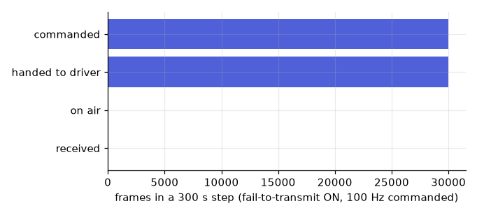
A paced sender has four counters for one step: frames commanded (slots times rate), frames handed to the driver, frames on air, and frames received. The sender's own counter is the second one. It counts calls that returned without error, not radiated frames. Only the receivers' count of the sender's frames proves transmission.
Worked step (300 s, 100 Hz, fail-to-transmit on, 6 % loss on a healthy path): commanded 30000, handed 30000, on air 0, received 0. The sender counter reports 100 % of commanded with zero errors; the delivered rate is 0.0 Hz. With the failure off, the same step delivers 28200 frames, 94.0 Hz.
Measured. One 2.4 GHz injector, nine receivers, steps of five minutes over several nights, on two 2.4 GHz channels. In 37 of 73 steps (50.7 %) none of the nine receivers heard a single injector frame, while the injector's counter reported a full count and zero errors. The receivers were alive: on one 2.4 GHz ladder, one receiver logged 14,356 to 26,755 frames from 40 to 53 other transmitters inside each silent step, against 7,151 of 7,503 injector frames in the 25 Hz step before. The injector's own receive path was also down in those steps, which is consistent with a radio bring-up that fails about half the time and leaves the card neither receiving nor transmitting; that mechanism is a hypothesis, not a finding. On a 5 GHz channel, 0 of 20 steps were silent, and delivery in the heard steps was flat between 0.958 and 0.979 from 25 to 500 Hz.
Consequence for analysis. A step in which no receiver heard the sender is an instrument failure, not a 0 % delivery. Pooling silent steps with heard ones produces a rate effect that is a bring-up failure: with an assumed healthy delivery of 0.95 (an assumption, not a measurement), counting the 37 silent steps as zeros gives a pooled mean of 0.468.
Concept check. The sender reports 30000 frames handed and 0 errors for a step. Three of nine receivers heard 25000 or more frames each; six heard none. What is the delivered rate and how do you treat the six? Answer: delivered rate is computed from receivers that heard the sender (about 83 Hz for a 300 s step with 25000 frames). The six are checked for a separate fault (deaf receivers, wrong channel) before they enter any average; the sender's counter plays no part.
4. Channel load, not physics
Two 5 GHz channels 20 MHz apart differ in wavelength by 0.38 %. Propagation does not separate them. If a band contrast is measured between two such channels and delivery differs, the cause is load.
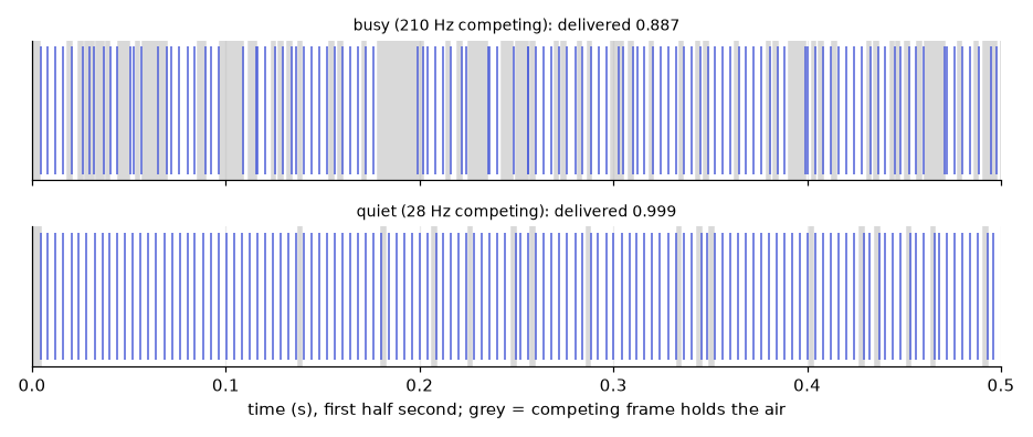
Mechanism sketch used in the widget: a 250 Hz injector (slot 4 ms) shares the channel with Poisson competing frames, each holding the air for an assumed 2 ms. The injector senses the channel at each slot start. If busy it waits, then draws a backoff of b_i nine-microsecond slots from 0..\text{CW}; a queued competitor draws b_c; equal draws collide and the injector frame is lost, the larger draw waits. A frame that cannot leave before its own slot ends is skipped. The 2 ms is an assumption (a monitor decodes only some of the frames it hears, so the real airtime is unknown), and nothing here is fitted to the measurement below.
Worked numbers (30 s window, CW 31, seed 7):
| Competing traffic | Air held | Delivered | Skipped | Collided |
|---|---|---|---|---|
| 28 Hz (quiet) | 0.056 | 0.999 | ||
| 210 Hz (busy) | 0.420 | 0.887 | 0.107 | 0.006 |
The gap is 0.113. Across competing traffic of 0, 100 and 300 Hz, delivery is 1.000, 0.984 and 0.718. The contention window trades two failures: at 210 Hz, CW 15 delivers 0.894 (collisions 0.011) and CW 127 delivers 0.821 (collisions 0.002, but more slots skipped because the waiting frame misses its slot).
Measured. One injector at 250 Hz on two 5 GHz channels (5.22 and 5.24 GHz), nine receivers, four 30-minute blocks in the order busy, quiet, quiet, busy. Delivery was the injector's frames counted at each receiver divided by the frames the injector handed to its driver (an acceptable denominator here because, on the 5 GHz channel checked, no step was silent at every receiver, unlike on 2.4 GHz). The busy channel carried about 210 Hz of access-point traffic; the quiet one about 28 Hz. Median delivery was 0.756 on the busy channel and 0.922 on the quiet one. The paired difference, receiver-level mean, was +0.141 with a cluster bootstrap 95 % interval of [+0.101, +0.178], positive at 9 of 9 receivers. One night in one building, so the interval covers receiver-to-receiver spread and nothing else. Delivery on the busy channel varied by 28 points across receiver positions and by 11 on the quiet one.
A related observation: passive capture rate on one busy 5 GHz channel moved between 97 and 800 Hz depending on the hour of the day.
Rule: before a band contrast is read as physics, measure competing traffic alongside, order conditions ABBA, and carry delivered rate as a covariate.
Concept check. A 2.4 GHz run delivers 61 Hz and a 5 GHz run delivers 99 Hz at the same commanded rate. Can you say 2.4 GHz propagation is worse? Answer: not yet. Band and load differ together. Measure competing traffic on both channels, and repeat on two 5 GHz channels of unequal load to see how large the load effect alone is.
5. Who transmitted?
An ambient stream pools many transmitters. There is a second trap: the receiver firmware writes one placeholder source address for broadcast frames that no known network owns. All such frames then share one address, though they come from an unknown number of transmitters. Any timing statistic must be scoped to one transmitter first.
Consecutive frames from a single transmitter cannot be closer than one frame airtime. A 200-byte frame at 6 Mb/s legacy OFDM takes about 292 microseconds (computed from the 802.11a symbol formula, assuming the 200 bytes are the whole PSDU). Adding the 5 GHz DIFS (34 microseconds) and a mean backoff of 7.5 slots of 9 microseconds raises the floor to about 394 microseconds (computed here); 292 is the conservative bound. A median gap well below that means several transmitters share the address.
Widget model: an injector at 250 Hz on a jittered grid (gap CV 0.04), six ambient transmitters at 15 Hz each (Poisson), and optionally placeholder-address frames (Poisson, 300 Hz). 10 s window, seed 7.
| Scope | Gap CV |
|---|---|
| Pooled, all frames (6445 frames) | 0.787 |
| Top address (the placeholder) | 0.955 |
| Injector address only | 0.040 |
A Poisson process has CV 1, a perfect grid has CV 0. Without placeholder frames and with one ambient transmitter, the pooled CV is 0.206; with six ambient transmitters and no placeholder, 0.470 and the most frequent address is the injector, so scoping by frequency happens to work. It stops working when the placeholder outnumbers the injector, which is the case above.
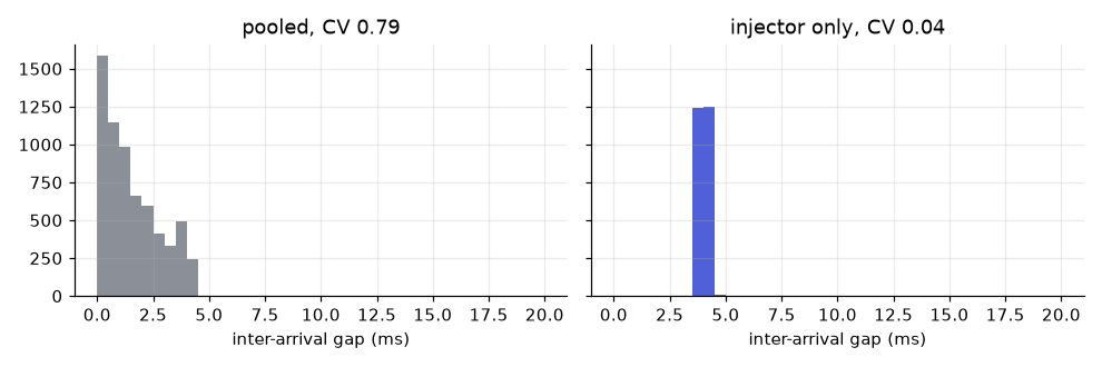
Measured. On a walk capture with the injector at about 250 Hz, gap CV was 0.999 when the analysis had scoped to the placeholder address and 0.04 after scoping to the injector's own address. In a separate one-hour 6 GHz capture, 88.1 % of records carried the placeholder address, and the next two addresses (6.0 % and 5.9 %) were the management radios of two receivers in the rig. Tells that an address is the placeholder: RSSI spread over tens of dB, frames near-field at some receivers and absent at others, and a median gap below the single-frame airtime.
Concept check. A capture has 88 % of records under one source address and a median gap of 173 microseconds. Is that one transmitter? Answer: no. 173 microseconds is below the airtime of a single 200-byte legacy frame (about 292 microseconds), so several transmitters share the address.
6. The 6 GHz band: a bursty pilot
A mean rate hides the arrival process. For Doppler, what matters is the largest gap the walker can slip through, because across a gap of length g the local Nyquist limit is
In words: a stream that averages 200 Hz but goes silent for 464 ms cannot follow a walker across that silence at any speed above a few centimetres per second.
Widget model: bursts of B frames, burst starts a Poisson process with rate 200/B so the mean stays near 200 Hz, gaps inside a burst exponential with median 172.7 microseconds. 60 s window, seed 7, wavelength at 5975 MHz (5.017 cm).
| B | Rate (Hz) | Median gap | p95 gap | CV | Longest gap |
|---|---|---|---|---|---|
| 1 (Poisson) | 203.2 | 3446 us | 14.7 ms | 1.00 | 46.8 ms |
| 4 | 204.3 | 252 us | 30.3 ms | 2.56 | 160.9 ms |
| 12 (default) | 201.0 | 187 us | 29.6 ms | 4.63 | 464.2 ms |
| 40 | 215.3 | 173 us | 0.9 ms | 8.32 | 865.4 ms |
At the default the mean rate would allow v_\text{max} = 2.521 m/s, the p95 gap allows 0.424 m/s and the longest gap allows 0.027 m/s. With periodic instead of random bursts (12 frames, 60 ms apart) the p95 gap is 57.2 ms and the longest gap is 59.1 ms, so the local limits are 0.219 m/s at the p95 and 0.212 m/s at the longest gap: same mean rate, an eight-fold higher floor on the longest-gap limit (0.212 against 0.027 m/s).
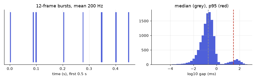
Measured. Ten receivers tuned to 5975 MHz (6 GHz preferred scanning channel, 20 MHz monitor width) for one evening hour; the figures are from one of them. Over the loaded window the receiver logged 199.7 Hz with a median gap of 172.7 microseconds, p95 28.5 ms, p99.9 102.6 ms and gap CV 3.58; every record was a legacy 52-tone record. Read with the local limit: the p95 gap allows 0.440 m/s and the p99.9 gap 0.122 m/s. The hour was one channel on one evening, followed by a retraction of an earlier verdict on the band: it is a pilot, and the record class in that hour says which frames yielded CSI, not that the band cannot yield other classes. Who sent the frames was not established (section 5).
Concept check. Two streams both average 200 Hz. One has gap CV 1.0 and one has 4.6. Which is safer for Doppler and why? Answer: the CV 1.0 stream (Poisson). Its longest gap is tens of milliseconds; the CV 4.6 stream sits silent for hundreds of milliseconds, and v_\text{max}(g) = \lambda/(4g) falls with the longest gap, not the mean.
7. The 802.11bf sensing session
The amendment moves sounding from opportunistic to negotiated. It applies to bands from 1 to 7.125 GHz, which includes 2.4, 5 and 6 GHz, and separately to bands above 45 GHz (du2025_5663 ↗); the sub-7 GHz procedure is described in ropitault2024_d49d ↗. The two corpus surveys were written before the amendment was final: one expected ratification by September 2024 (ropitault2024_d49d ↗) and the other expected publication in March 2025 (du2025_5663 ↗). The course log records it as published in 2025; that date was not confirmed against a primary source for this lecture.
The sub-7 GHz procedure has four steps: capabilities exchange, sensing measurement session setup, sensing measurement exchange, and termination (du2025_5663 ↗). The other survey splits it into five phases (session setup, measurement setup, measurement instances, measurement setup termination, session termination). Roles are orthogonal: the sensing initiator starts the procedure and a sensing responder answers; independently, a sensing transmitter sends the NDP and a sensing receiver measures it. An NDP (null data packet) carries training fields and no payload; it reuses the sounding frame already defined for beamforming, so the PHY does not change.
Trigger-based (TB) instance. The initiator is an AP and one or more clients respond. The phases, in order, are polling, NDPA sounding, trigger-frame (TF) sounding and optional reporting:
- The initiator sends a Sensing Polling TF. Each responder that is available answers with CTS-to-self, one SIFS later, multiplexed by OFDMA. A responder in power save may not reply.
- NDPA sounding (downlink): the initiator sends an NDPA naming its recipients, then an SI2SR NDP; the recipients measure it.
- TF sounding (uplink): the initiator sends a trigger frame; the responders send SR2SI NDPs, multiplexed spatially; the initiator measures them.
- Reporting: measurement results return in a report, immediately or delayed.
A responder that did not answer the poll does not take part in the sounding phases that follow. Non-TB instance. The initiator is a client and the responder is one AP. There is no polling phase, because an AP never enters power save. The client sends an NDPA to the AP, then an SI2SR NDP one SIFS later; the AP answers with an SR2SI NDP within SIFS; in the optional reporting phase the AP sends a Sensing Measurement Report a SIFS after its NDP. The exchange is the same for uplink, downlink or both, and it is limited to bistatic sensing (ropitault2024_d49d ↗).
Frame bookkeeping in the widget (simplified: every replying responder is both a downlink receiver and an uplink transmitter, one NDP serves all downlink receivers, the uplink NDPs share one slot):
| Responders | Frames with report | Channel accesses with report | Frames without report |
|---|---|---|---|
| 1 | 8 | 8 | 6 |
| 2 | 11 | 9 | 8 |
| 3 | 14 | 10 | 10 |
| 4 | 17 | 11 | 12 |
If one of three responders does not answer the poll, 2 are sounded and the exchange is 11 frames. A non-TB exchange is 4 frames with a report and 3 without. For scale, a CTS-to-self of 14 bytes at 6 Mb/s lasts 44 microseconds and SIFS on 5 GHz is 16 microseconds.
Why this matters for rate. In a TB session the AP sets the interval between instances, so the sounding rate is a parameter of the session, not of the neighbours' traffic. Section 2's ceiling then becomes a scheduling requirement: the instance rate must exceed 4v/\lambda for the fastest target of interest. A multi-link device can sense on several bands (2.4, 5 and 6 GHz), and the survey notes that the uncompressed CSI feedback then grows with each band added (du2025_5663 ↗).
Concept check. In a trigger-based instance with three responders, one never answers the poll. What changes? Answer: it is not sounded and sends no NDP and no report; 2 responders are sounded and the instance is 11 frames instead of 14.
8. What a standard report costs
The report carries the channel frequency response between each transmit and receive antenna, each value scaled and quantised, with the scale factors included; CSI is the only measurement the amendment defines (ropitault2024_d49d ↗). Values are encoded in 8 or 10 bits and only 1 of every 4, 8 or 16 tones is reported (grouping). The uncompressed CSI matrix is the only feedback type adopted, so overhead grows with bandwidth (du2025_5663 ↗). The widget's grid (grouping 1, 2, 4, 16; 4, 6, 8, 10 bits) is a teaching grid that goes beyond the standard's values on purpose, so the student can see why those values were chosen.
In words: two real numbers (real and imaginary part) of b bits for every reported tone; NMSE is the error energy as a fraction of the channel energy, in dB (more negative is better). The receiver rebuilds unreported tones by linear interpolation.
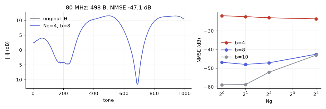
Synthetic channel used in the widget: 8 paths with exponential delays (mean 50 ns), exponentially decaying gains, tone spacing 78.125 kHz, seed 11. HE tone counts: 242, 484, 996 and 1992 at 20, 40, 80 and 160 MHz. Raw reference: complex float, 8 bytes per tone.
Worked numbers, 80 MHz (996 tones; amplitude range across the band 23.2 dB):
| Grouping | 4 bits | 6 bits | 8 bits | 10 bits |
|---|---|---|---|---|
| 1 | -21.9 dB, 996 B | -34.8 dB, 1494 B | -46.9 dB, 1992 B | -58.9 dB, 2490 B |
| 2 | -22.4 dB, 498 B | -36.1 dB, 747 B | -48.0 dB, 996 B | -58.8 dB, 1245 B |
| 4 | -23.0 dB, 249 B | -36.2 dB, 374 B | -47.1 dB, 498 B | -52.2 dB, 623 B |
| 16 | -23.6 dB, 63 B | -35.6 dB, 95 B | -42.6 dB, 126 B | -43.0 dB, 158 B |
The default (grouping 4, 8 bits) reports 249 tones in 498 bytes against 7968 raw, 16 times smaller, at -47.1 dB. Two regimes appear. At few bits, quantisation noise dominates and grouping costs nothing (about -23 dB at 4 bits regardless of grouping). At many bits, interpolation error dominates: at 10 bits, grouping 16 sits at -43.0 dB against -58.9 dB with no grouping. Grouping slightly improves NMSE at 8 bits (interpolating two quantised neighbours averages their errors), which is an artefact of this channel and quantiser. This channel is smooth (short delay spread); a channel with longer delay spread raises the interpolation floor.
Bandwidth scales the price directly. At grouping 4 and 8 bits: 122 B at 20 MHz, 242 B at 40 MHz, 498 B at 80 MHz, 996 B at 160 MHz (NMSE -50.4, -47.7, -47.1 and -47.0 dB). Sounding 160 MHz with no grouping and 10 bits gives 4980 B per antenna pair at -57.2 dB; for a 2 by 2 link reporting 100 times per second that is 15.94 Mb/s of feedback. The default 80 MHz configuration at the same rate costs 1.594 Mb/s. The earlier version of this week gave -42.3 dB for grouping 4 with 8 bits on a different synthetic channel; the two values are not comparable.
Concept check. At 100 Hz on a 2 by 2 link with 160 MHz, how much does a report at grouping 4 and 8 bits save over no grouping and 10 bits, and what does it cost in error? Answer: 996 B against 4980 B per pair, a 5-fold reduction (about 3.19 Mb/s against 15.94 Mb/s). On the 160 MHz synthetic channel the error rises from -57.2 dB to -47.0 dB; whether that matters depends on the task, and the standard's own grouping and bit values are 4, 8 or 16 tones and 8 or 10 bits.
Where the standard stops
The report is the channel frequency response as measured. The surveys read for this lecture describe scaling factors for the quantiser but do not describe a receiver gain state, a phase correction or a calibration step; that description is from the surveys, not from the amendment text. The physical causes are not removed by a report format: carrier and sampling frequency offsets give random phase offsets that differ from packet to packet (zhang2022_5822 ↗), and at 4000 frames per second a 100 kHz offset can move the phase by up to 50\pi between consecutive values (wang2015_48cf ↗). Week 5 starts from a stream whose timing is known and scoped to one transmitter and shows the ladder that makes its phase and amplitude usable. The same holds whether the stream came off a patched card or an 802.11bf session.
The uneven sampling of data frames is a separate, documented problem: CSI taken from data frames has an uneven sampling interval because packet arrival is random (zhang2022_5822 ↗). Scheduling by session is the standard's answer to it.
Exam questions
1. Derive the ceiling on measurable speed for packet rate PRR and wavelength \lambda. What does a walker at 1.0 m/s look like at 40 Hz on 5.2 GHz? The echo rotates at f_D = 2v/\lambda. Packets sample it, so the phase step per packet is 2\pi f_D/\text{PRR}, which must stay below \pi. That gives |f_D| < \text{PRR}/2 and v_\text{max} = \lambda\text{PRR}/4. At 5.2 GHz, \lambda = 5.765 cm and f_D = 34.69 Hz. At 40 Hz, v_\text{max} = 0.577 m/s, so the line folds to ((34.69 + 20) \bmod 40) - 20 = -5.31 Hz: a walker of about -0.153 m/s, slow and reversed. With magnitude-only data the sign is lost as well.
2. A sender reports 30000 frames handed to the driver and no errors in a 300 s step. What can you conclude about the delivered rate? Nothing. The counter records calls that returned, not frames on air. In a measured set of 73 steps on 2.4 GHz, none of nine receivers heard the injector in 37 while its counter showed a full count. Delivered rate comes from receivers that heard the sender's address; a step in which none heard is an instrument failure and is excluded, not averaged in as zero. Delivered rate uses received frames over duration (28200/300 = 94.0 Hz in the healthy example).
3. Two channels 0.4 % apart in wavelength deliver 0.756 and 0.922 of an injector's frames. Is that band physics? How would you design the next experiment? No, the wavelength difference leaves no propagation explanation. The difference is consistent with load: the busy channel carried about 210 Hz of access-point traffic against about 28 Hz. The paired difference of +0.141 with interval [+0.101, +0.178] over nine receivers excludes zero for this night and building. The next design measures competing traffic on each channel, orders conditions ABBA to cancel drift, includes at least two channels of unequal load in the same band, and reports delivered rate as a covariate before any band contrast is read.
4. A stream averages 200 Hz with gap CV 3.6 and a p95 gap of 28.5 ms. Give the local Doppler ceiling at 5975 MHz for the mean rate and for the p95 gap, and say what you would report. Mean rate: v_\text{max} = \lambda \cdot 200/4 = 0.05017 \times 50 = 2.51 m/s. p95 gap: \lambda/(4 \times 0.0285) = 0.44 m/s. The gap distribution, not the mean, sets what can be followed. Report the median, p95 and longest gap, the CV, and the local limit at the p95 and at the longest gap; a mean rate alone is not a sufficient description. The p99.9 gap of 102.6 ms gives 0.122 m/s.
5. An 802.11bf trigger-based instance has four polled responders and one does not answer. List the phases and say which frames each responder sends. Polling: the initiator sends a Sensing Polling TF; three responders send CTS-to-self (multiplexed by OFDMA). NDPA sounding: the initiator sends an NDPA and an SI2SR NDP; the three responders measure. TF sounding: the initiator sends a trigger frame and the three responders send SR2SI NDPs (spatially multiplexed); the initiator measures. Reporting (optional): a report trigger, then reports from the three. The fourth responder sends nothing in any phase. In the simplified count that is 1 + 3 + 1 + 1 + 1 + 3 = 10 frames without reporting and 14 with it.
6. A 160 MHz report with no grouping at 10 bits, 2 by 2 antennas, 100 reports per second. Compute the feedback rate and name the two knobs that shrink it. Per antenna pair 2 \times 10 \times 1992/8 = 4980 bytes; four pairs at 100 per second is 4980 \times 4 \times 100 \times 8 = 15.94 Mb/s. The knobs are grouping N_g (report every N_g-th tone) and bit depth b. Grouping 4 with 8 bits reduces it to 996 bytes per pair, about 3.19 Mb/s. The price is reconstruction error: on the 160 MHz synthetic channel, -47.0 dB against -57.2 dB.
Further reading
- du2025_5663 ↗: the four-step procedure, TB and non-TB exchanges, feedback types, multi-link sensing.
- ropitault2024_d49d ↗: roles, phases, report quantisation and grouping, client-based sensing.
- ropitault2024_db32 ↗: the velocity ceiling written for the 60 GHz passive case.
- soumya2023_9b9f ↗: the radar form V_\text{max} = \lambda/(4T_c).
- wang2016_6482 ↗: torso and leg Doppler bands from CSI spectrograms.
- zhang2022_5822 ↗: uneven sampling, unsynchronised transceivers.
- wang2015_48cf ↗: carrier frequency offset and the frame-rate ceiling of a commodity card.
- zhu2024_472f ↗: the one sounding-rate sweep found in the corpus.
- zhang2025_72c4 ↗: sampling rate of an open 802.11ax CSI tool.
- li2022_4220 ↗: CSI at 1 kHz next to passive radar.
- wang2022_2397 ↗: survey with the qualitative velocity-ambiguity statement.
Provenance (instructor only)
First-party numbers in this lecture and where they were read:
.claude/memory/illumination-and-injector.md: injection frame format and rates; forced OFDM rate on 2.4 GHz; injector counter semantics; 61.3 and 99.4 Hz deliveries, pooled CVs 0.714 and 0.083, two-thirds dead-slot share; 12 transmitters on the 5 GHz capture; placeholder-address behaviour and its tells; scoped CV 0.999 to 0.04..claude/memory/csi-doppler-rate-floor.md: walking bands and the Nyquist rate for the legs; the one rate-sweep paper; the design-rule attribution (checked against the papers: the radar form is in soumya2023_9b9f and ropitault2024_db32, wang2022_2397 states it only qualitatively).obsidian/monad-knowledge/diary/2026-09-03 - The 6 GHz band answered on the third try at 200 records a second, and the lake's decoder is two days behind the fleet.md: the 6 GHz hour (199.7 Hz, median gap 172.7 microseconds, p95 28.5 ms, p99.9 102.6 ms, CV 3.58, legacy 52-tone records, 88.1 % placeholder address), the delivery comparison of the two 5 GHz channels (0.756, 0.922, +0.141 [+0.101, +0.178], 9 of 9, 28 and 11 point spreads, 210 and 28 Hz traffic), the 37 of 73 silent 2.4 GHz steps and the flat 5 GHz delivery.obsidian/monad-knowledge/diary/2026-09-04 - The 6 GHz verdict was not supportable, and the lake tools were racing on one connection.md: the retraction (one pilot hour, no verdict) and the 97 to 800 Hz range of passive capture rate by hour of day. That diary calls the swing about 4x; the endpoints differ by 8.2x and this lecture quotes only the range..claude/memory/ax210-pi5-driver.md: 5 GHz AP mode is impossible on the card (firmware gate), so illumination is monitor-mode injection..claude/memory/illumination-and-injector.mdalso gives the 394 microsecond single-source floor; this lecture derives it as airtime plus DIFS plus mean backoff, which is an interpretation, not stated on the page.obsidian/monad-knowledge/diary/2026-09-03 - The 6 GHz band answered on the third try at 200 records a second, and the lake's decoder is two days behind the fleet.md(Addendum 2): the live-receiver check on a silent step (14,356 to 26,755 ambient frames from 40 to 53 transmitters; 7,151 of 7,503 in the preceding 25 Hz step).obsidian/monad-knowledge/edu/courses/WS501-wifi-csi-sensing/WS501 Curriculum.md: the course-log line recording publication of the amendment in 2025 (not confirmed against a primary source).