How to use this note
The deck is the primary material: each concept is one live widget with its controls, a picture, the formula with the current values substituted, a one-line readout and an "In words:" gloss. This note is the reader companion, in the deck's order. It holds the derivations, the worked numbers, the concept checks and the exam questions.
Every number below is printed by workbook.ipynb (numpy, scipy and matplotlib only, executed) and stored in numbers.json. A widget at its default state runs the same formula, defaults and seed as the workbook cell, so it shows the same number. The random numbers come from a small seeded generator (mulberry32 with Box-Muller), reimplemented in the workbook in integer arithmetic; a "draw" is one seed, not a different experiment.
Week 1 ended with the log-distance model and a warning that the shadowing term is large. This week treats the model as an instrument: three parameters to fit, a calibration that goes stale, and failure modes that are reproducible in a few lines of code. The course model from week 1 is P(d_0) = -59 dBm at d_0 = 1 m, n = 3, \sigma = 6 dB. Week 1 gave the linearised ranging error \sigma_d \approx 0.46\,d.
Vocabulary that joins this week:
- Least squares: choose the line whose summed squared vertical misses are smallest. The model is a straight line on a log-distance axis, so this is all the fitting machinery needed.
- Residual: measurement minus fitted line. Its spread estimates \sigma.
- Bias vs scatter: scatter changes from reading to reading, bias stays. Averaging attacks scatter only.
- Lever arm: the spread of calibration points along log-distance, S_{xx} in decades squared. A slope fitted over a short lever arm is mostly noise.
Motivating case. Exposure-notification apps treat a phone as a risky contact when signal strength puts it within 1 to 2 m for 10 to 20 minutes, and the same paper that describes this calls signal strength "a rather poor proxy for being in close contact" (hoepman2022_1ae5 ↗). This week computes how poor a proxy a decibel is, and what a calibration can and cannot repair. The corpus does not carry independent field measurements of that attenuation, so the case stays a motivation, not a data source.
1. Free space: the one number you can compute
Start with an isotropic transmitter of power P_t. At distance d the power has spread over a sphere of area 4\pi d^2:
A receiving antenna harvests P_r = S(d)\,A_e with effective aperture A_e = G_r \lambda^2 / (4\pi). Combining,
In decibels, with powers in dBm and gains in dB,
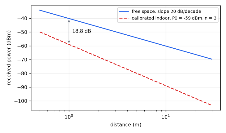
The isotropic free-space path loss is (4\pi d/\lambda)^2 in bensky2019_6c00 ↗ (Eq. 2.12). \mathrm{FSPL} is a straight line in \log_{10} d with slope 20 dB per decade, which is 10n with n = 2. In free space n = 2 is a theorem. Everywhere else it is a fitted parameter.
In words: free space loses 6 dB every time the distance doubles, because a sphere's area quadruples.
Worked numbers (workbook section 1, 2.44 GHz, 0 dBm, isotropic antennas):
| Quantity | Value |
|---|---|
| wavelength \lambda = c/f | 12.29 cm (12.3 cm) |
| \mathrm{FSPL}(1\ \mathrm{m}) | 40.20 dB |
| P_r(1\ \mathrm{m}) | -40.20 dBm |
| gap to the course reference -59 dBm | 18.80 dB |
| loss per doubling, n = 2, 3, 4 | 6.02, 9.03, 12.04 dB |
| loss per doubling, n = 1.215 | 3.66 dB |
| 1 m to 16 m in free space | 24.08 dB |
The wavelength enters through the aperture, not through absorption: at a higher frequency the same gain corresponds to a smaller collecting area.
Why P(d_0) is measured. The course reference sits 18.80 dB below the free-space prediction at 1 m. The Friis form assumes lossless matched antennas, a known transmit power and no environment. A real phone has none of these, and the transmit power of a given phone is not known to the receiver. The reference therefore has to be measured in place. huang2023_7523 ↗ states the same requirement: the reference value and the exponent are empirical, tied to hardware and environment, and must be calibrated in the application environment. One BLE positioning system in the corpus computes its reference at d_0 = 0.8 m with the free-space model, chooses n and X_\sigma per scenario from a cited recommendation, and compares this against an empirical model whose 1 m reference is measured (cantnpaterna2017_8af8 ↗).
Break it (widget). Invert an observed -80 dBm with the Friis value -40.20 dBm instead of -59 dBm, at n = 3. The calibrated inversion gives 5.01 m, the Friis one gives 21.22 m: the distance is multiplied by 10^{18.80/30} = \times 4.23. The mistake does not look like noise; it is a scale factor that no averaging removes.
2. The exact price of a decibel
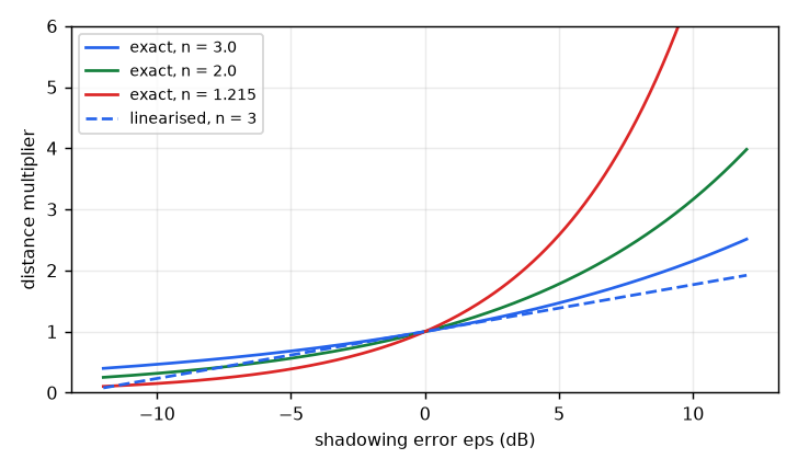
Invert the mean model. From P_\mathrm{obs} = P(d_0) - 10 n \log_{10}(\hat d/d_0),
Let the reading be \varepsilon dB below the mean at the true distance, P_\mathrm{obs} = P(d_0) - 10n\log_{10}(d/d_0) - \varepsilon. The mean-model terms cancel:
In words: a decibel error multiplies the distance by a factor that depends only on the error divided by the exponent.
Three consequences.
- Only \varepsilon/n matters. 4 dB at n = 2, 6 dB at n = 3 and 8 dB at n = 4 all give \times 1.585.
- Exponential growth. 8 dB at n = 2 gives \times 2.512 = 1.585^2.
- Asymmetry. +\varepsilon multiplies and -\varepsilon divides. At the default of the widget (d = 5 m, n = 3, \varepsilon = \pm 6 dB) the estimate is 7.92 m for +6 dB and 3.15 m for -6 dB, factors \times 1.585 and \times 0.631. A symmetric dB error is a right-skewed metre error. The median of \hat d / d is 1 (the median of \varepsilon is 0), so a CDF of ranging error keeps an unbiased p50 and grows a long upper tail: at n = 3, \sigma = 6 dB the p10 and p90 factors are \times 0.554 and \times 1.804.
Week 1's linearisation gave a one-sigma error of \ln 10\cdot\sigma/(10n) = 0.46\,d. The exact one-sigma excess at the same parameters is 10^{6/30} - 1 = 0.585. The linear form is the tangent; the exact factor overtakes it as \varepsilon/n grows.
| \varepsilon (dB) | n | exact factor | linearised |
|---|---|---|---|
| 4 | 2 | 1.585 | 1.460 |
| 6 | 3 | 1.585 | 1.460 |
| 8 | 2 | 2.512 | 1.921 |
| 8 | 4 | 1.585 | 1.460 |
| 2.86 | 1.215 | 1.720 | 1.542 |
| 2.63 | 1.215 | 1.646 | 1.498 |
| 1 | 1.215 | 1.209 | 1.190 |
| 6 | 1.2 | 3.162 | 2.151 |
A low exponent is bad for ranging. The pair (\sigma, n) = (2.86\ \mathrm{dB}, 1.215), measured in an open hall (section 6), gives \times 1.72 per sigma, worse than the noisy canonical office (\times 1.585), and its p90 factor is \times 2.00. The steeper the fade, the more decibels each metre buys.
3. Fitting P(d0), n and sigma by least squares
The model is a line in x = \log_{10}(d/d_0):
Minimise J(a,b) = \sum_i (y_i - a - b x_i)^2. Setting both partial derivatives to zero gives the normal equations, and dividing the first by N gives \bar y = a + b\bar x. Then
In words: the slope of the line is the exponent, its height at 1 m is the reference power, and its scatter is the error carried into every range.
Two degrees of freedom are spent on the line, so the residual variance divides by N-2 (devore2012_62c8, section 12.3). At the widget default the residual SD with divisor N would be 4.14 dB against 4.18 dB with N-2.
P(d_0) and n set the mean curve; errors in them are systematic and correctable. \sigma passes through the section 2 factor and bounds accuracy.
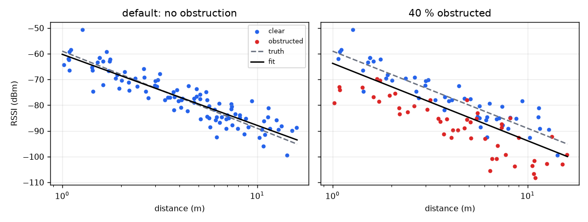
The default state. P_0 = -59 dBm, n = 3, \sigma = 4 dB, 100 readings log-uniform over 1 to 16 m, no obstruction, draw 1. The fit returns \hat P_0 = -60.23 dBm, \hat n = 2.764, \hat\sigma = 4.18 dB, one-sigma factor \times 1.417. The sampling SD of \hat n here is \sigma/(10\sqrt{S_{xx}}) = 0.125 with S_{xx} = 10.17 decades squared, so this draw sits 1.9 SD below the truth. That is a property of the draw. Over 200 further draws the mean \hat n is 2.995 (SD 0.124) and the mean \hat\sigma is 3.985 dB. The five draws of the widget's draw selector exist to show this.
Obstruction (break it). Add 40 % of readings that carry an extra 10 dB loss (iannizzotto2022_1c98 ↗ relays about 10 dB for a body on the line of sight, from a 2014 experiment; the extra-spread of 4 dB here is an assumption of this workbook) and fit one model to the pool. A pooled fit cannot know which readings were obstructed. The mixture variance is
so \sigma_\mathrm{pool} = 6.81 dB. The widget draw gives \hat\sigma = 7.13 dB, \hat P_0 = -63.74 dBm, \hat n = 3.010 (49 obstructed of 100), factor \times 1.725. Over 200 draws \hat\sigma averages 6.80 dB (factor \times 1.69 with the mean \hat n) and \hat n averages 2.985.
That last number answers "did n go up or down?": with obstruction independent of distance, the extra loss shifts the intercept and inflates \hat\sigma, and leaves the slope unbiased. If obstruction becomes likelier with distance (the widget's toggle: share rising from 0 at 1 m to twice the set share at 16 m), the extra loss grows with distance and the fitted exponent rises: the widget draw gives \hat n = 3.442 and \hat\sigma = 6.23 dB, and the 200-draw means are \hat n = 3.586, \hat\sigma = 5.72 dB. No radio changed. zhuang2016_a6e9 ↗ states the same trap: a model fitted from all LOS and NLOS training data may not work for either, and the paper replaces it with a polynomial regression.
Small N. At N = 5 the five draws give \hat\sigma = 4.40, 3.74, 2.17, 2.38, 3.57 dB and \hat n = 2.70, 3.91, 3.91, 2.50, 2.74 against a true 4 dB and 3. A five-point fit is a coin toss on both.
4. The lever arm: where you stand when you calibrate
For a fixed set of calibration distances the slope estimate has variance \mathrm{Var}(\hat b) = \sigma^2/S_{xx} with S_{xx} = \sum (x_i - \bar x)^2 (devore2012_62c8: spread-out x values give a more precise slope). Since b = -10n,
In words: precision comes from spread along log-distance, not from the number of points, and a slope measured over a short stretch is mostly noise that is multiplied when it is extrapolated.
Design. The room truth is P_0 = -60.5 dBm, n = 3.25, \sigma = 6 dB. The old model is (-59\ \mathrm{dBm}, 3.0). Each of 400 trials draws K calibration readings, refits, and inverts noise-free mean readings at 11 distances over 4 to 14 m. The score is the median relative error |\hat d - d|/d. The old model scores 0.327 (its error is purely the parameter mismatch).
| K and placement | S_{xx} (decades^2) | sd(\hat n) analytic | sd(\hat n) over trials | median rel. error, refit |
|---|---|---|---|---|
| 3, log-spaced 1 to 2 m (default) | 0.045 | 2.82 | 2.80 | 0.610 |
| 12, log-spaced 1 to 2 m | 0.107 | 1.83 | 1.87 | 0.505 |
| 3, log-spaced 1 to 12 m | 0.582 | 0.79 | 0.78 | 0.193 |
| 3, at 1, 4, 12 m | 0.585 | 0.79 | 0.78 | 0.191 |
| 6, log-spaced 1 to 12 m | 0.815 | 0.67 | 0.65 | 0.161 |
| 12, log-spaced 1 to 12 m | 1.376 | 0.51 | 0.52 | 0.122 |
| 3, crowded in the nearest quarter of 1 to 12 m (in log) | 0.036 | 3.15 | 3.12 | 0.650 |
The default is already the broken state. Three points at 1 to 2 m span 0.30 decades, \mathrm{sd}(\hat n) = 2.8 is as large as the exponent itself, and the extrapolated lines fan out over the evaluation band: the re-fit (0.61) loses to the old model (0.33). The same three points at 1, 4 and 12 m cover 1.08 decades, S_{xx} is 13 times larger, and the re-fit wins (0.19). Quadrupling the points to K = 12 in the same 1 to 2 m range raises S_{xx} only 2.4 times, to 0.107, and the re-fit still loses (0.505). Widening the range at fixed K raises S_{xx} with the square of the log-range. More points still help across a fixed range (0.161 to 0.122 from K = 6 to 12 over 1 to 12 m), but the lever arm dominates.
A published ladder can be priced the same way. sadowski2020_f2ba ↗ measured RSSI at 18 distances, every 0.1 m from 0 to 1 m and every 0.5 m from 1 to 5 m, and fitted n and C per technology and scenario. Reading that as one reading per distance from 0.1 to 5 m (0 m has no logarithm), S_{xx} = 4.17 decades squared and \mathrm{sd}(\hat n) = 0.29 at 6 dB. The passage does not state the readings per distance and its Table II values are not in the corpus index, so this is a price of the design, not a claim about the paper's results. cantnpaterna2017_8af8 ↗ used 0.5 to 5 m in 0.5 m steps with 500 readings per step.

Week 10 turns this into a schedule; the constraint any recalibration schedule must respect is the lever arm.
5. One model, two rooms: why a fit drifts
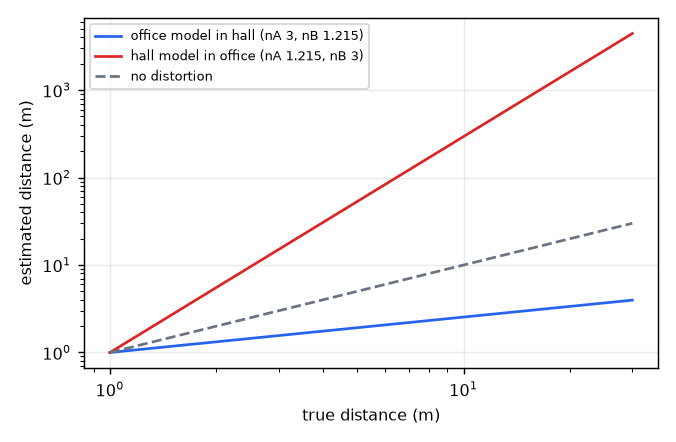
A model fitted in room A, (P_{0A}, n_A), inverting readings that come from room B, (P_{0B}, n_B). The reading at true distance d is P_{0B} - 10 n_B \log_{10} d. The inversion with A's parameters solves P_{0A} - 10 n_A \log_{10}\hat d = P_{0B} - 10 n_B \log_{10} d:
In words: an exponent mismatch bends distances as a power law, and a reference mismatch scales them by a constant.
| Case | \hat d at 2, 5, 10, 20 m |
|---|---|
| office model (n_A = 3) in a hall (n_B = 1.215), no offset, exponent ratio 0.405 | 1.32, 1.92, 2.54, 3.36 m |
| hall model in an office (ratio 2.469) | 5.54, 53.2, 295 m at 2, 5, 10 m |
| equal exponents (n = 3), offset +6 dB | factor \times 1.585 at every distance |
| equal exponents, offset -6 dB | factor \times 0.631 |
| equal exponents, 40 % obstructed in B | factor \times 1.359 (mean extra loss 0.4 \cdot 10 dB, assumed to act as an offset) |
At the default a phone 10 m away in the hall looks 2.54 m away, a factor 0.25. Swapping the rooms turns 5 m into 53 m. The swap is not symmetric because a power law with ratio above 1 explodes.
The deployed-system version of this is the change of the propagation mixture over time: a door now closed, a shelf now full, a room now occupied. A single fit silently redistributes the change into P_0, n and \sigma (section 3). This is the mechanism the week demonstrates on synthetic data. The corpus does not quantify what share of field drift it explains, so the note claims a mechanism, not a share. The corpus supports per-room, per-technology fits (sadowski2020_f2ba ↗), the requirement to calibrate in the application environment (huang2023_7523 ↗), and lists a changing environment among the causes of lower positioning accuracy of a single measurement (guo2020_267f ↗, challenges section).
6. An exponent below free space: the open hall
Scenario. Ten Bluetooth receivers sit at about 90 cm height around one open hall. A phone at roughly chest height is carried on a 25 minute walk, and nine of the ten receivers hear it. The median RSSI of each receiver in each 2 s bin is paired with the horizontal distance that a reference track gives; pairs closer than 1 m are dropped, and one log-distance model is fitted. It is calibrated on the same walk it is later scored on, so it is optimistic. The fit is P_0 = -62.11 dBm, n = 1.215, \sigma = 2.86 dB from 5,468 pairs.
Reading the exponent. A textbook table lists free space 2, open field 4, in-building line of sight 1.6 to 1.8 and in-building obstructed 4 to 6 (bensky2019_6c00 ↗, Table 2.1, citing a standard text). 1.215 is below free space and below the in-building line-of-sight row. One BLE system lists channelling of energy, especially in corridors, among indoor propagation effects (cantnpaterna2017_8af8 ↗). The corpus is silent on a measurement paper that derives or measures a waveguide-like exponent below 2 in a hall; the two pointers above are all it holds, and the fit is one hall. The fitted value also depends on the fit design, as the next paragraphs show.
Consequence for ranging. Loss per doubling is 10 \cdot 1.215 \log_{10} 2 = 3.66 dB, and the one-sigma factor is 10^{2.86/12.15} = \times 1.72. In words: a hall that funnels energy loses only 3.7 dB per doubling, so each decibel of noise moves the distance estimate further. Small \sigma does not compensate for small n. A reference taken from Friis at 1 m would be -40.20 dBm; the gap to -62.11 dBm is 21.91 dB and would multiply distances by \times 63.6 at n = 1.215. This gap is not all propagation, because the phone's transmit power is unknown.
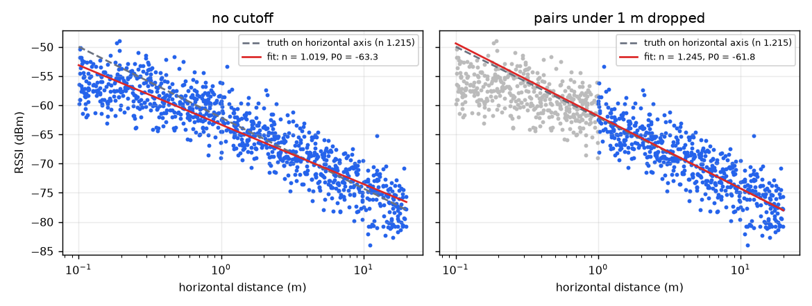
Geometry trap. The receiver sits about 0.3 m below the phone but the regression uses the horizontal distance d_h, which is what a floor plan knows. The slant distance is \sqrt{d_h^2 + v^2}, so the ratio slant to horizontal is \sqrt{1 + (v/d_h)^2}: 1.044 at 1 m and 1.414 at 0.3 m for v = 0.3 m. The closest pairs have the most leverage on P_0. In the real walk, 86 of 5,651 pairs lay inside 0.3 m, which is why pairs under 1 m are dropped.
The widget simulates this with an assumption stated on its slide: horizontal distances log-uniform over 0.1 to 20 m (a wider share of near pairs than the real walk), P_0 = -62.11 dBm, \sigma = 2.86 dB, 1000 pairs, true n = 1.215, fit on the horizontal distance.
| vertical offset | cutoff | \hat n | \hat P_0 (dBm) | pairs dropped |
|---|---|---|---|---|
| 0 m (control) | 0 | 1.209 | -62.05 | 0 % |
| 0.3 m | 0 | 1.019 | -63.32 | 0 % |
| 0.3 m (default) | 1.0 m | 1.245 | -61.83 | 42.6 % |
| 1.0 m | 0 | 0.708 | -65.84 | 0 % |
| 1.0 m | 1.0 m | 1.151 | -62.76 | 42.6 % |
With no cutoff, the near pairs (weaker than the horizontal distance predicts) flatten the line: \hat n falls and \hat P_0 falls. The 42.6 % dropped share follows from the assumed log-uniform draw. At the other regimes of the widget (true n = 2, 1.7, 5; offset 0.3 m, cutoff 1 m) the fit returns 2.022, 1.725 and 4.993, so with the cutoff in place the geometry costs little in this simulation.
7. What averaging can and cannot buy
Split the dB error at a fixed spot into per-packet fading and shadowing that is frozen for that spot. Fading changes over wavelength-scale moves and over time as people move (bensky2019_6c00 ↗); shadowing "fundamentally limits the accuracy of RSSI-based ranging" (fallani2026_04be ↗). Averaging N packets divides the fading variance by an effective count and leaves the shadowing untouched:
for AR(1)-correlated packets with correlation \rho (the large-N approximation). In words: waiting longer at one spot removes the flicker, never the spot's own offset.
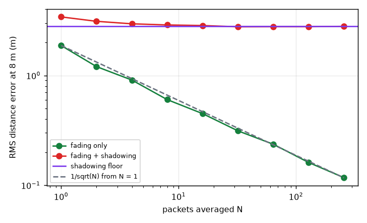
Widget default: 64 packets, \sigma_f = 3 dB, \sigma_s = 4 dB, true distance 8 m, n = 3, 400 seeded positions.
| RMS distance error at 8 m | N = 1 | N = 64 |
|---|---|---|
| fading only | 1.871 m | 0.236 m |
| fading and shadowing | 3.411 m | 2.779 m |
| shadowing floor (limit N \to \infty) | 2.799 m |
The fading-only curve follows the 1/\sqrt{N} prediction (0.234 m at N = 64). The realistic curve flattens onto the floor. The total at N = 64 is 0.02 m below the floor because both are sample values on the same 400 positions. The formula gives \sigma_\mathrm{eff} = \sqrt{16 + 9/64} = 4.02 dB, factor \times 1.361 at n = 3.
Break it: with \sigma_s = 0 averaging works to the bottom (1.871 m to 0.117 m at N = 256); with \sigma_f = 0 it does nothing (2.799 m at N = 1 and N = 256); with \rho = 0.9, N_\mathrm{eff} = 3.37 and 64 packets give a fading-only error of 0.944 m, which is what 3 independent packets give (1.033 m; 1.871/\sqrt{3.37} = 1.020).
Teaser for week 7. The dB-domain version of this is the dwell test. In an open-hall walk with position fixes solved from at least three receivers per 2 s bin, the walker stood still at 29 places for a median of 21 fixes. The error of one fix at a stop was 2.87 m and after averaging the stop it was 2.84 m, where white noise would have given 0.63 m. The hall's own 2.86 dB residual is a residual of 2 s bin medians, so it is already mostly floor.
8. Per-receiver reference powers: removing a mixture, and what it buys
Receivers and phones differ in reference level. Pooling them into one P_0 puts the offset variance into \sigma:
for J offsets evenly spaced over a range R (an assumption for the widget). In words: giving each receiver its own reference level removes the part of the scatter that belongs to the receiver, not the part that belongs to the room.
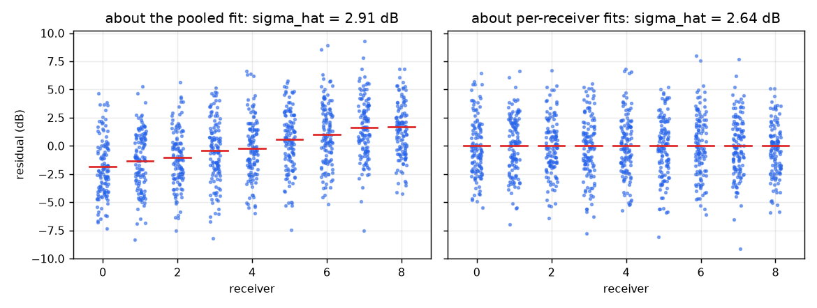
Default: J = 9, R = 3.7 dB, shadowing \sigma = 2.63 dB, 600 readings per receiver, exponent for the multiplier 1.215.
- Analytic: \mathrm{Var} = 1.426 dB^2, \sigma_\mathrm{pooled} = 2.888 dB.
- Simulation: pooled \hat\sigma = 2.906 dB (factor \times 1.734), per-receiver \hat\sigma = 2.640 dB (factor \times 1.649), a 9.2 % reduction. Fitted offsets span 3.545 dB against the true 3.7.
- Held-out (fit on the first half of each receiver's readings, RMS residual on the second half): with 600 readings per receiver, pooled 2.954 dB and per-receiver 2.677 dB. With 5 readings per receiver, pooled 3.060 dB and per-receiver 3.448 dB (factors \times 1.786 and \times 1.922): the per-receiver model scores worse. In-sample it does not look better either after the degrees-of-freedom correction (2.684 pooled, 2.803 per-receiver dB), so the held-out split is what shows it.
The hall, stated in place. In the open-hall walk, fitting one reference power per receiver on 5,467 pairs gave a spread of 3.71 dB (the largest offsets +2.82 and +2.01 dB) and cut the residual from 2.86 to 2.63 dB, 7.9 %. Whether 3.71 dB is a range or an SD is not stated in the source; the widget treats it as a range. The analytic pooled value at the default, 2.89 dB, is consistent with the measured 2.86 dB, which does not prove the offsets are evenly spaced. Fitted on one half of the walk and scored on the other, the median position error moved by -0.24 m in one fold and +0.03 m in the other while the p90 fell by 1.37 m and 0.47 m (3.70 m and 8.48 m global against 3.46 m and 7.11 m per receiver; 1.82 m and 4.98 m against 1.85 m and 4.51 m). The offsets buy the tail, not the median. What remains is the room itself, which a two-parameter model cannot hold.
The same mechanism at channel level. zhuang2016_a6e9 ↗ reports per-channel means and SDs of one static beacon at 5 m (channel 37: -71.9 dBm, SD 2.4; channel 38: -68.1, SD 0.8; channel 39: -78.8, SD 2.7) and uses separate models per channel. Pooling the three with equal weights (an assumption) gives an SD of 4.92 dB. iannizzotto2023_86c7 ↗ notes that commodity receivers cannot tell which advertising channel a packet used, so this pooling cannot be undone from the reading alone. Week 4 owns channels.
Hand-off
- Week 3 (multi-anchor positioning in an open hall): the input range uncertainty is the one-sigma factor 10^{\sigma/(10n)}; the pair to carry is (n, \sigma) = (1.215, 2.86\ \mathrm{dB}), factor \times 1.72. In the RSS position-error bound of liu2022_9677 ↗ the squared position error bound is proportional to the shadowing variance and inversely proportional to the square of the path-loss exponent.
- Week 4: channels are only pointed at here (section 8).
- Week 7: the averaging floor is the dB-domain version of the dwell test.
- Week 10: the lever arm of section 4 is the constraint for any recalibration schedule.
Exam-Style Questions
Q1 (derivation). Starting from the received-power form of the log-distance model, derive the relation between a shadowing error of \varepsilon dB and the resulting distance estimate. Evaluate the one-sigma factor for (a) \sigma = 8 dB, n = 4 and (b) \sigma = 8 dB, n = 2, and state the p90 factor at n = 3, \sigma = 6 dB. Model answer. Invert the mean model, substitute P_\mathrm{obs} = P_\mathrm{mean}(d) - \varepsilon, and the mean terms cancel to \hat d = d\,10^{\varepsilon/(10n)}. (a) \sigma/n = 2 gives \times 1.585; (b) \sigma/n = 4 gives \times 2.512. Only \sigma/n enters, the dependence is exponential, and halving n squares the factor. The p90 of \varepsilon is 1.2816\,\sigma, so the p90 factor is 10^{1.2816 \cdot 6/30} = \times 1.804, and the p10 factor is \times 0.554.
Q2 (Friis and the reference). Derive \mathrm{FSPL}(d) = 20\log_{10}(4\pi d/\lambda) and state the physical origin of each factor. Compute the wavelength and \mathrm{FSPL}(1\ \mathrm{m}) at 2.44 GHz. Give two reasons why a phone's measured 1 m reference sits below the free-space prediction, and say what happens to a range if the Friis value is used with n = 3. Model answer. Sphere gives P_t G_t/(4\pi d^2); aperture A_e = G_r\lambda^2/(4\pi); combine and take -10\log_{10}. \lambda = 12.29 cm and \mathrm{FSPL}(1\ \mathrm{m}) = 40.20 dB. Reasons: non-isotropic lossy detuned antennas, unknown transmit power, environment (floor, body) already present at 1 m; any two argued. The gap to -59 dBm is 18.80 dB, so the distance is multiplied by 10^{18.80/30} = \times 4.23 (5.01 m becomes 21.2 m at -80 dBm).
Q3 (the purchase order). A facilities team calibrates a beacon system in an empty building and obtains \hat n = 2.99, \hat\sigma = 4.0 dB. Six months later a monitoring script refits live data and reports \hat n = 2.99, \hat\sigma = 6.8 dB. The team concludes the beacons are failing and orders replacements. Argue against the order: which mechanism explains the numbers without a hardware change, what would distinguish it, and what would you measure? Model answer. An obstruction mixture. In the workbook, 40 % of readings with an extra 10 dB loss and 4 dB extra spread lift the 200-draw mean \hat\sigma from 3.99 to 6.80 dB (analytic 6.81 dB) and leave \hat n at 2.985, and the one-sigma factor rises from \times 1.36 to \times 1.69. The signature is inflated \hat\sigma with a stable exponent. If obstruction grows with distance, \hat n rises too (3.59, with \hat\sigma 5.72 dB); which one applies is a question about where the obstructed readings sit. To confirm, refit on a clear-line subset or a short re-sweep at a few distances: if the clear residuals are still near 4 dB, the hardware is unchanged. Also state the limit: this is a synthetic mechanism, and the same numbers could come from other causes.
Q4 (averaging floor). With 3 dB per-packet fading and 4 dB shadowing at 8 m (n = 3), averaging 64 packets moves the RMS distance error from 3.41 m to 2.78 m. Explain why it stalls, what the floor consists of, and name two interventions that go below it. Model answer. Averaging divides the fading variance by N_\mathrm{eff} (fading-only 1.87 m to 0.24 m, the 1/\sqrt{N} line) but the shadowing offset is identical in every packet. The floor (2.80 m) is the shadowing error alone. Below it: spatial diversity (several receivers or positions re-draw the shadowing, turning bias into scatter that can be averaged) and a better model or a second modality (attack the bias). With \rho = 0.9, N_\mathrm{eff} = 3.37, so correlated packets average worse still.
Q5 (lever arm). Using \mathrm{Var}(\hat n) = \sigma^2/(100\,S_{xx}), explain why K = 3 points at 1 to 2 m gave a worse model (median relative error 0.61) than keeping the mismatched old model (0.33), why the same three points at 1, 4 and 12 m gave 0.19, and why 12 points at 1 to 2 m gave only 0.51. Model answer. Three points at 1 to 2 m cover about 0.3 decades, S_{xx} = 0.045, \mathrm{sd}(\hat n) = 6/(10\sqrt{0.045}) = 2.8, and the slope is extrapolated to 4 to 14 m. At 1, 4, 12 m, S_{xx} = 0.585 and \mathrm{sd}(\hat n) = 0.79. 12 points at 1 to 2 m give S_{xx} = 0.107, \mathrm{sd}(\hat n) = 1.83. The lever arm counts, not the number of points.
Q6 (a hall that ranges badly). A hall fit gives n = 1.215, \sigma = 2.86 dB; an office fit gives n = 3, \sigma = 6 dB. Which ranges better per sigma, and what does a mismatch between the two do to a distance? Which fit-design choice moved the hall exponent in the simulation? Model answer. The office: \times 1.585 against \times 1.72. Using the office model in the hall maps d to d^{0.405} (10 m reads as 2.54 m); the reverse maps 5 m to 53 m. Including pairs closer than 1 m with a 0.3 m vertical offset lowered \hat n from 1.245 to 1.019 and \hat P_0 from -61.83 to -63.32 dBm, because horizontal distance understates slant distance most where the pairs are closest.
Further Reading
- bensky2019_6c00 ↗: Friis form (Eq. 2.12), the exponent table (Table 2.1), the log-distance model with a Gaussian shadowing term (Eq. 2.14).
- sadowski2020_f2ba ↗: per-room, per-technology curve fits and a calibration ladder to price by S_{xx}.
- cantnpaterna2017_8af8 ↗: log-distance model with shadowing chosen per scenario; corridor channelling.
- zhuang2016_a6e9 ↗: LOS and NLOS mixtures break one fitted model; per-channel means.
- iannizzotto2022_1c98 ↗ and iannizzotto2023_86c7 ↗: body occlusion (relayed), channel-blind receivers.
- devore2012_62c8: slope variance and N-2 degrees of freedom.
- fallani2026_04be ↗: shadowing limits RSSI ranging.
- guo2020_267f ↗ and huang2023_7523 ↗: changing environments and calibrating in place.
- roy2022_18d3 ↗: the log-distance model in survey form.
- liu2022_9677 ↗: forward pointer for week 3, the position error bound versus \sigma and n.
- hoepman2022_1ae5 ↗: signal strength as a proximity proxy.
The corpus is silent on the original Friis paper, the original Okumura and Hata papers, and on spatial correlation of shadowing (week 6 will need it as textbook material or an assumption). Textbook background without a corpus source: the free-space transmission formula carries Friis's name; the empirical path-loss tradition of Okumura and Hata fitted measurements to closed forms.
Provenance (instructor only)
Vault and repository paths behind the first-party numbers in sections 6, 7 and 8 and the course model:
- diary/2026-09-09 - Filtering the BLE track removes the bounce and cannot remove the miss, because two thirds of the miss is a bias fixed to the room.md
- monad_knowledge/web/static/lab/fiit-ground-0.json (repository file, model block: -62.11 dBm, 1.215, 2.86 dB, 5,468 pairs, in-session calibration)
- monad_knowledge/web/lab_atlas.py (repository file: 2 s bins, at least 3 receivers per fix, the 1 m calibration cutoff, receiver and phone heights, 86 of 5,651 pairs inside 0.3 m)
- edu/courses/LOC502-ble-rf-localization/week-01-rf-ranging-fundamentals-rssi-tof/lecture.md (course model -59 dBm, n = 3, \sigma = 6 dB; linearised 0.46\,d)
Open item: hall dimensions differ between the course scenario note and the survey-walk polygon; they are not quoted here.