This is the reader companion to the interactive deck. It follows the deck's order. Every number in it is printed by workbook.ipynb (run it to reproduce them) and stored in numbers.json. A widget in the deck at its default state shows the same number as the workbook, because it uses the same formula, the same defaults and the same seeded generator. Nothing here is a measurement unless a line says so.
0. Where we are, and a few words first
Ranging means estimating how far away a radio transmitter is from something you can measure at the receiver. Three things can be measured: how strong the signal is (RSSI), how long it took (time of flight, ToF), and which way it came from (angle of arrival, AoA). Each one buys geometry and each one has a price. This week states both prices in metres.
- dBm: power on a logarithmic scale. +10 dB is a factor of ten in power.
- Anchor: a radio at a known position.
- Path loss: how much weaker the signal is after travelling. It grows with distance.
- Shadowing: random extra weakening from walls, furniture and bodies, different at every spot.
Torch intuition. Step twice as far from a torch and the same light spreads over four times the area. In open air the received power falls by 10 log10(2^2) = 6.02 dB per doubling of distance (path-loss exponent n = 2). Indoors the fade is steeper. At n = 3 each doubling costs 9.03 dB (workbook s1).
Sign convention. This is the most common week-1 error. Path loss PL grows with distance. Received power P falls with distance. They are the same physics with opposite signs: P = P_ref - PL. This course always reports the received power P.
1. Strength as a ruler: invert the log-distance model
RSSI measures amplitude only. The mean model, with shadowing X_sigma as a zero-mean Gaussian in dB, is
The course canonical values are P_0 = -59 dBm, n = 3 and sigma = 6 dB. Week 2 quotes them. Invert the mean model to get a range from a reading:
One standard deviation of shadowing multiplies or divides the range by
In words: one standard deviation of dB noise stretches or shrinks the range by the same factor at every distance. The factor depends on sigma/n only, so (4 dB, n = 2) and (6 dB, n = 3) give the same 1.585 (workbook s1).
Worked numbers at d = 5 m: the mean power is -79.97 dBm, the +/- sigma band is -85.97 to -73.97 dBm, and the interval is 3.15 to 7.92 m. Of 20 seeded readings at 5 m, 14 land inside that bracket (70 %, against 68 % expected for one sigma). Break it: at sigma = 10 dB and n = 1.5, F = 4.64 and the interval at 5 m is 1.08 to 23.2 m, wider than the room. At sigma = 0, F = 1 and the bracket collapses.
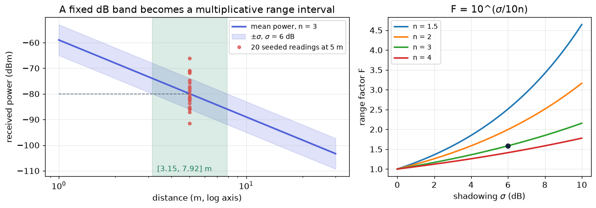
Shadowing is frozen in space. It depends on where the transmitter and receiver stand, not on when you read, so repeated readings at one spot repeat the same offset. Week 2 separates it from per-packet fading and finds the floor that averaging cannot pass; week 6 treats how far one must move to change it. Multipath shadowing blurs the monotonic RSSI trend and limits RSSI ranging (fallani2026_04be ↗, qualitative). Bluetooth uses forty 2 MHz channels (bensky2019_6c00 ↗; iannizzotto2022_1c98 ↗). That fact matters in section 3.
2. Why the error grows with distance, and why the mean range is long
Differentiate the inversion with respect to the observed power:
In words: the metres-per-dB conversion is proportional to the distance already reached, like a rubber band that is harder to control the further it is stretched. At n = 3 and d = 10 m it is 0.768 m per dB (a central-difference check gives the same value). Replace the perturbation by sigma:
That is 2.30 m at 5 m and 4.61 m at 10 m. Error is multiplicative because the model is logarithmic in distance.
The exact interval is asymmetric. At 10 m it runs +5.85 m and -3.69 m, against a linearised +/-4.61 m. The range estimate d_hat = d 10^(-sigma Z/(10n)) is log-normal. Exponentiating a symmetric dB error keeps the median at d, so the inverted range is median-unbiased. Its mean is
which is 11.2 % long in the mean. A simulation of 10^6 draws gives a mean ratio of 1.111 and a median ratio of 0.999, consistent with 1 (workbook s2). Averaging ranges in metres therefore overestimates them. This asymmetry is the source of the right-skewed metre errors in section 6.
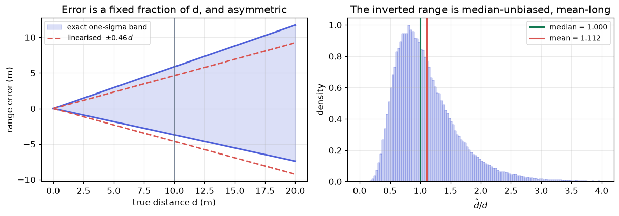
Break the linearisation: at sigma = 10 dB and n = 1.5 the linearised error at 10 m is 15.4 m, while the exact band is +36.4 m and -7.85 m. The linear line stops being honest when sigma/n is large.
3. Time of flight: a delay is a distance, if the clock and the bandwidth allow
Distance is d = c tau, so 1 ns of timing error is 0.2998 m. One-way time of arrival needs clocks synchronised at both ends. Two-way ranging cancels the offset:
This is eq. 14.4 in bensky2019_6c00 ↗. The IEEE 802.11 fine timing measurement uses it and gives sub-metre Wi-Fi location (same source). With a 100 ns clock offset, one-way ranging of a 10 m link returns 39.98 m (30.0 m of bias), and the two-way formula returns 10.00 m (workbook s3).
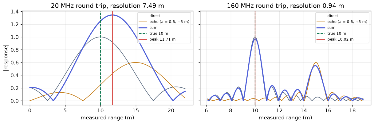
Resolution. A pulse of bandwidth B has a delay main lobe about 1/B wide. The range resolution is therefore c/B one way and c/(2B) round trip. This is a derivation. The corpus states only the radar form c/2B (ropitault2024_d49d ↗), which also gives WLAN sensing resolutions of 0.5 to 10 m because of the narrow bandwidth.
| bandwidth | one way c/B | round trip c/2B |
|---|---|---|
| 2 MHz (one Bluetooth channel) | 149.9 m | 74.9 m |
| 20 MHz | 14.99 m | 7.49 m |
| 40 MHz | 7.49 m | 3.75 m |
| 80 MHz | 3.75 m | 1.87 m |
| 160 MHz | 1.87 m | 0.94 m |
| 499.2 MHz (a high-rate-pulse UWB channel) | 0.60 m | 0.30 m |
For one 2 MHz channel, 1/B = 500 ns. A 2 MHz Bluetooth channel therefore cannot range a room by time. The 499.2 MHz figure is the nominal bandwidth of the sub-gigahertz UWB channel in bensky2019_6c00 ↗.
Resolution is not accuracy. The corpus bound improves with SNR and with the squared effective bandwidth, and multipath interferes with the estimate of the first arrival unless the first path is resolvable (liu2022_9677 ↗). A non-line-of-sight path always adds a positive range bias (same source). Indoors the line-of-sight assumption behind TOA and TDOA does not hold, because of multipath and non-line-of-sight propagation (guo2020_267f ↗), so a blocked direct path makes the first detected arrival an echo. The workbook models one echo of relative amplitude a = 0.6 that arrives 5 m later in measured range, in phase with the direct pulse, and finds the peak of |sinc((r - r0)/dr) + a sinc((r - r0 - Delta)/dr)| with dr = c/(kB) on a 1 mm grid. This is an assumption, not a measurement.
| bandwidth (round trip) | resolution | peak pulled by the 5 m echo |
|---|---|---|
| 2 MHz | 74.9 m | +1.874 m |
| 20 MHz | 7.49 m | +1.710 m |
| 40 MHz | 3.75 m | +0.268 m |
| 80 MHz | 1.87 m | +0.067 m |
| 160 MHz | 0.94 m | +0.016 m |
| 499.2 MHz | 0.30 m | +0.002 m |
One-way at 20 MHz the same echo pulls the peak by +1.841 m. A 30 m echo at 20 MHz one way lands on a sidelobe and biases the peak negative, -1.224 m. Bandwidth sets how close two paths can be before they merge into one wrong peak, and the clock sets a bias that no bandwidth removes.
The same modulo trap appears in phase-based ranging: the phase of the arriving wave fixes the distance only up to a whole number of wavelengths, and two frequencies differing by less than c/d remove the ambiguity (bensky2019_6c00 ↗, eqs. 14.7 and 14.8). The corpus is silent on Bluetooth channel sounding, so this week does not treat it.
4. Angle of arrival: phase across two antennas, and the ghost angles
A plane wave reaches two antennas spaced d apart with a path difference d sin(theta). The phase difference and the bearing are
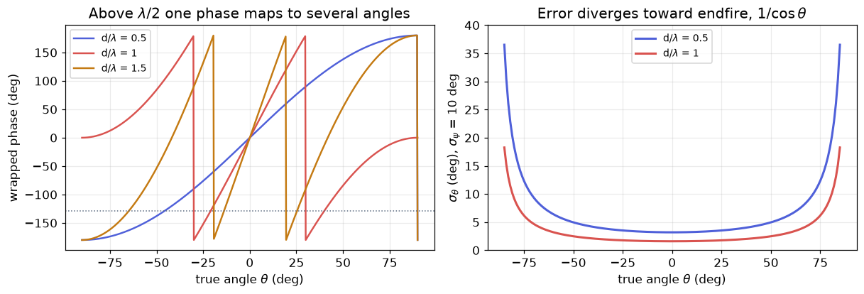
(iannizzotto2022_1c98 ↗, eq. 1; the same phase shift (2 pi/lambda) d sin(theta) appears in abedi2022_cdad ↗). The receiver sees psi only modulo 2 pi. For d/lambda of at most 1/2, every sin(theta) in [-1, 1] maps to a unique wrapped phase. Above 1/2, several angles share one phase, so the candidates are sin(theta_m) = (psi_w + 2 pi m)/(2 pi d/lambda) inside [-1, 1]. This is the textbook aliasing rule. The corpus does not state it explicitly.
At 2.44 GHz, lambda = 12.29 cm and lambda/2 = 6.14 cm. At 5.2 GHz, lambda = 5.77 cm and lambda/2 = 2.88 cm (workbook s4). At the default d/lambda = 0.5 and theta = 30 degrees, psi = 90.0 degrees, theta_hat = 30.0 degrees, and there is one candidate.
Ghosts. At d/lambda = 1.0 and theta = 40 degrees, psi = 231.4 degrees, which wraps to -128.6 degrees, and theta_hat = -20.9 degrees. Two candidates, -20.9 and 40.0 degrees, give the same phase. At d/lambda = 1.5 and 30 degrees there are three, -56.4, -9.6 and 30.0 degrees. Avoid d/lambda = 1.0 at exactly 30 degrees as an example: psi = 180 degrees sits on the wrap edge.
Noise and endfire. With phase noise sigma_psi,
The error is smallest broadside and diverges toward endfire, where the derivative of the phase difference is zero (liu2022_9677 ↗). At sigma_psi = 10 degrees and d/lambda = 0.5, sigma_theta = 3.68 degrees at 30 degrees, which is 0.64 m across at 10 m (0.32 m at 5 m). At 80 degrees it is 18.3 degrees, or 3.20 m across at 10 m, and at 85 degrees it is 36.5 degrees. Wider spacing sharpens the angle, 1.84 degrees at d/lambda = 1.0, until it aliases.
Bluetooth 5.1 adds a Constant Tone Extension so that an antenna-switching receiver can measure this phase (iannizzotto2022_1c98 ↗). The corpus reports no measured Bluetooth 5.1 AoA accuracy figure. Two bearing lines from two array-equipped anchors fix a 2D position (guo2020_267f ↗; bensky2019_6c00 ↗). For arrays beyond two elements and for the ambiguity of the general case, see schmidt1986_8a38 ↗.
5. What each measurement costs and buys, on one scale
At a common true distance of 5 m (sigma = 6 dB, n = 3, 20 MHz round trip, d/lambda = 0.5, sigma_psi = 10 degrees, theta = 30 degrees):
| measurement | uncertainty in metres | what it costs | anchors for a 2D fix |
|---|---|---|---|
| RSSI | interval 3.15 to 7.92 m, 4.77 m wide | one commodity antenna, no clock | 3 |
| ToF | resolution 7.49 m, plus any echo or clock bias | bandwidth; synchronised clocks one way, or two-way exchanges | 3 (TDoA: synchronised references, and a fourth station for a unique fix) |
| AoA | +/-0.32 m across the bearing, and no range at all | an antenna array at each anchor | 2 |
At 10 m the RSSI interval is 6.31 to 15.85 m (9.54 m wide) and the AoA cross-range is 0.64 m. The ToF resolution does not depend on distance. The anchor counts follow bensky2019_6c00 ↗ (circles from three stations; TDoA needs a fourth) and guo2020_267f ↗ (two array-equipped anchors). The cheapest measurement is the least precise, and the precise ones pay in bandwidth, clocks or antennas.
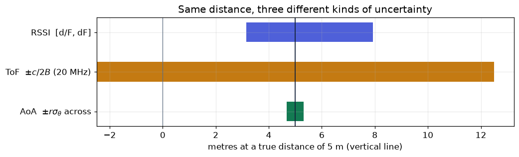
Break it: at d/lambda = 1.2 a ghost falls inside +/-85 degrees and the angle becomes ambiguous (two candidates). At B = 2 MHz the ToF resolution is 74.9 m and the bar leaves the room.
Literature anchors, each with its own setup, not a like-for-like ranking:
- A UWB indoor positioning system with error below 0.3 m, at high power consumption and high cost (cantnpaterna2017_8af8 ↗).
- WLAN sensing range resolution of 0.5 to 10 m because of the narrow bandwidth (ropitault2024_d49d ↗).
- Commodity Wi-Fi with 3 antennas and 40 MHz resolves only a few tens of degrees and a few metres (zhang2026_956c ↗).
- RSSI trilateration averaged over BLE, Wi-Fi and ZigBee gave 2.71, 2.82 and 4.25 m in three rooms, and 3.26 m overall (sadowski2020_f2ba ↗).
6. Report the distribution
A range error from log-normal shadowing is right-skewed in metres:
The RMSE mixes scale and shape. From this week on, this course reports the empirical CDF with the median (P50) and the 90th percentile (P90) side by side, and the RMSE and mean only beside them. The analogy is commute times: if most trips take 20 minutes and a few take 90, the average looks fine until the day you hit a 90. The corpus offers examples of the reporting form and no methodological argument for it. A device-free UWB localiser (three sensors, an outdoor target area 5.5 m across) reads its ECDF at 50 % and 80 %, 0.64 m and 1.98 m (cimdins2022_fc11 ↗).
At d = 5 m, sigma = 6 dB and n = 3 the analytic values are median 1.51 m, P90 4.03 m and RMSE 2.76 m. At 2 m they are 0.61, 1.61 and 1.10 m, and at 10 m 3.03, 8.05 and 5.52 m. The seeded sample (Lcg seed 7, N = 500) gives median 1.49 m, P90 3.92 m, RMSE 2.67 m and mean signed error +0.45 m. The analytic mean signed error is +0.56 m, which is the 11 % mean bias of section 2 seen in metres. About 34 % of the readings fall within 1 m.
In words: half the ranges are within 1.5 m, one in ten is off by nearly 4 m, and no single number says both.
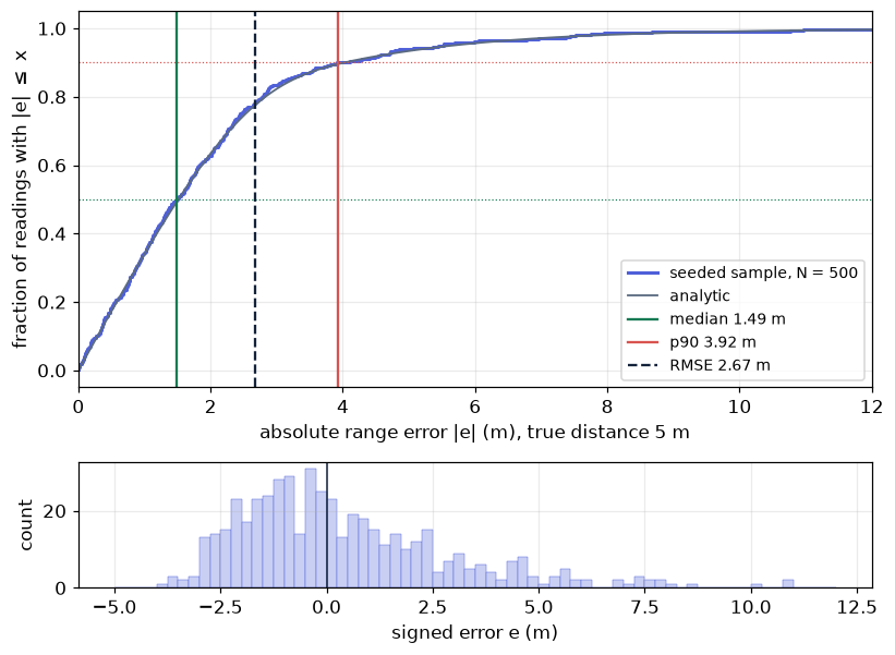
Break it with a small sample: at N = 20, the P90 over seeds 1 to 9 ranges from 2.53 to 5.86 m, while the analytic value stays at 4.03 m. At N = 500 the range over the same seeds is 3.79 to 4.61 m. A P90 from a small sample needs its own interval (a later week).
7. Break the single number: outliers and the same-RMSE impostor
Suppose a share of the readings loses an extra 10 dB, for example from a body or a wall in the path. Received power is lower, so those ranges are all too long:
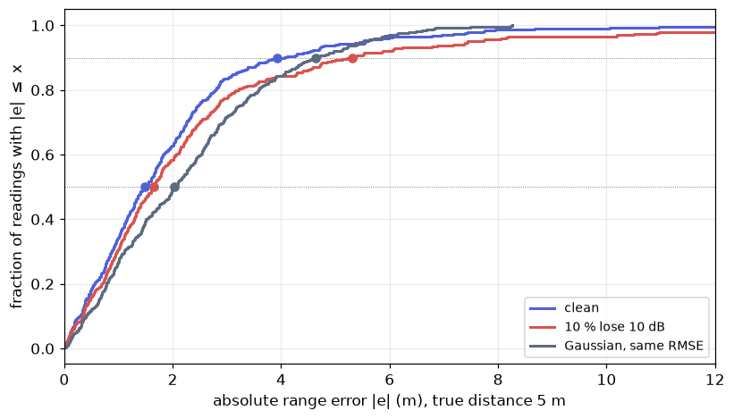
With s = 10 % (flags from a separate Lcg(11) stream, realised share 10.8 %) and L = 10 dB, on the same 500 readings as section 6:
| statistic | clean | with outliers | change |
|---|---|---|---|
| median | 1.49 m | 1.65 m | +0.15 m |
| P90 | 3.92 m | 5.32 m | +1.40 m |
| RMSE | 2.67 m | 3.81 m | +1.13 m |
Outliers live in the tail. The median barely notices them. The RMSE and the P90 move far more.
The impostor. A Gaussian-in-metres system with its scale set to the clean RMSE, 2.67 m (Lcg(23), N = 500), has median 2.04 m and P90 4.64 m. The 500 values drawn happen to have a sample RMSE of 2.83 m, so the RMSE match is by design of the scale and not exact in the sample. The point stands either way: an RMSE alone cannot tell two systems apart, and the median and P90 differ.
Breakdown point. At 15 dB the median itself moves as the share grows. With nominal shares of 0, 10, 20, 30, 40 and 50 % the median is 1.49, 1.69, 1.81, 2.14, 2.67 and 3.69 m. At 30 % (realised 28.0 %) the P90 is 13.58 m and the RMSE 8.36 m. A robust statistic is not immune to outliers. Its bias grows with the outlier share, and it fails completely at its breakdown point, the largest share it can tolerate. For the median the breakdown point is 50 %, where the outliers become the majority.
8. One real hall, reported honestly
Setup: ten Bluetooth receivers stand around a library hall and one adjoining room. A phone carried on a 1523.9 s walk is heard by nine of them, 155,034 readings in all. One position is solved every 2 s from one fitted path-loss model, 758 positions in total. The position error has median 2.48 m and P90 7.96 m, a P90 to median ratio of 3.2. These four values are quoted from a separate analysis, not computed in the workbook.
Set beside it the default single-range sample of section 6: median 1.49 m, P90 3.92 m, ratio 2.6. The first is a position error from many ranges and the second is one range at 5 m, so only the reporting form is compared. Why the median of the hall walk does not fall is the subject of weeks 7 and 8. The fitted exponent belongs to week 2.
Bridge to week 2. The factor F depends on sigma and n. Next week fits them.
Exam questions
- Derive the range factor. Invert the log-distance model, state F and the one-sigma interval, and explain why the error is multiplicative. Model answer: d_hat = d0 10^((P0 - P)/(10n)). A shadowing offset X shifts P by X, so d_hat = d 10^(-X/(10n)). One sigma of X gives the factor F = 10^(sigma/(10n)) and the interval [d/F, dF]. The interval scales with d because the model is logarithmic, so the same dB noise costs the same fraction of the distance at every range. At sigma = 6 and n = 3, F = 1.585 and sigma_d is about 0.46 d.
- Bias. At (6 dB, n = 3), is the inverted range biased? Model answer: median-unbiased, because a symmetric dB error exponentiates to a log-normal with median d. The mean is d exp(s^2/2) with s = sigma ln10/(10n) = 0.4605, so 1.112 d, 11.2 % long. Averaging ranges in metres overestimates them. At 10 m the exact interval is +5.85 and -3.69 m against a linearised +/-4.61 m.
- Why not time? Why can a 2 MHz Bluetooth channel not range a room, and what does a clock offset do? Model answer: the delay main lobe is about 1/B = 500 ns wide, so c/B = 149.9 m one way and c/2B = 74.9 m round trip. Any echo within that distance merges with the direct path. A clock offset of 100 ns adds c times 100 ns = 30.0 m to one-way ranging. Two-way ranging cancels the offset, because d = c[(t4 - t1) - (t3 - t2)]/2, but not the resolution limit.
- Ghosts. Two antennas at d/lambda = 1.0 see theta = 40 degrees. What does the receiver conclude, and why? Model answer: psi = 2 pi sin 40 degrees = 231.4 degrees, seen as -128.6 degrees. The estimate is arcsin(-128.6/360) = -20.9 degrees, and 40.0 degrees gives the same wrapped phase. Two candidates exist because the spacing exceeds lambda/2. At 2.44 GHz the safe limit is 6.14 cm. Near endfire the error also grows as 1/cos(theta): 3.68 degrees at 30 degrees and 18.3 degrees at 80 degrees for sigma_psi = 10 degrees and d/lambda = 0.5.
- Choose a signal. A deployment uses phones and coin-cell tags with one antenna and no clock synchronisation. Which measurement is available, how many anchors does a 2D fix need, and what error should you expect at 10 m? Model answer: RSSI. Three anchors for trilateration. The interval at 10 m is 6.31 to 15.85 m for (6 dB, n = 3). Time of flight would need bandwidth and two-way exchanges, and angle of arrival an array at each anchor (two anchors).
- Reporting. Two systems have the same RMSE of 2.67 m. What else must you report and why? Model answer: the median and the P90, ideally the whole CDF. In the workbook the log-normal range system has median 1.49 m and P90 3.92 m, and a Gaussian system scaled to the same RMSE has median 2.04 m and P90 4.64 m. Outliers move the RMSE and the P90 (2.67 to 3.81 m and 3.92 to 5.32 m at a 10.8 % share of 10 dB losses) far more than the median (1.49 to 1.65 m).
Exercises in the workbook
- Steeper n, smaller error? At sigma = 6 dB and d = 10 m, n = 2, 3, 4 give F = 1.995, 1.585, 1.413, median |e| of 4.39, 3.03, 2.30 m and P90 of 14.24, 8.05, 5.77 m. Larger n shrinks ln10/(10n), so a dB of noise buys fewer metres.
- When does the spread overwhelm the room? The linearised sigma_d first exceeds 5 m at d = 10.9 m for sigma = 6 dB, and at 6.5 m for sigma = 10 dB (n = 3).
What the corpus does not say
- No explicit derivation of the RSSI range Jacobian or of the factor 10^(sigma/(10n)). This note teaches it as a textbook derivation.
- The one-way c/B against round-trip c/2B distinction for link ranging is not stated. The corpus gives c/2B in radar form and two-way TOA timing.
- The lambda/2 spacing rule for unambiguous two-element AoA is not stated explicitly.
- No measured Bluetooth 5.1 AoA accuracy figure, and no Bluetooth channel sounding, was found.
- No methodological source argues for CDF or percentile reporting over RMSE. The corpus offers only examples.
Further reading
- guo2020_267f ↗: the measurement taxonomy (RSS, TOA, TDOA, AOA), two array-equipped anchors for AoA, NLOS for time methods.
- bensky2019_6c00 ↗: two-way TOA, TDOA and the fourth station, phase-of-arrival ambiguity, AOA geometry, BLE channels, HRP UWB at 499.2 MHz.
- ropitault2024_d49d ↗: range resolution c/2B and the 0.5 to 10 m WLAN figure.
- liu2022_9677 ↗: the TOA bound against SNR and effective bandwidth, DOA against d/lambda, broadside and endfire.
- iannizzotto2022_1c98 ↗: Bluetooth 5.1 direction finding and the Constant Tone Extension.
- sadowski2020_f2ba ↗: trilateration averages in three rooms, a single-number report to critique.
- cimdins2022_fc11 ↗: an error reported from ECDF percentiles.
- zhuang2016_a6e9 ↗: builds channel-separate models for the three advertising channels and finds the log path-loss model inaccurate indoors. Week 4 owns the channel story.
- schmidt1986_8a38 ↗: optional, array ambiguity and MUSIC beyond the two-antenna case.
Provenance (instructor only)
- obsidian/monad-knowledge/diary/2026-09-09 - Filtering the BLE track removes the bounce and cannot remove the miss, because two thirds of the miss is a bias fixed to the room.md (table row "raw, as published": median 2.48 m, P90 7.96 m; walk of 1523.9 s, 758 fixes, 155,034 readings on 9 of 10 nodes)
- obsidian/monad-knowledge/edu/courses/LOC502-ble-rf-localization/LOC502 Curriculum.md ("Scenarios the weeks may use": ten receivers around a library hall and one adjoining room; a course note, not a primary record)
- obsidian/monad-knowledge/edu/courses/LOC502-ble-rf-localization/week-01-rf-ranging-fundamentals-rssi-tof/workbook.ipynb (every computed number above)
- obsidian/monad-knowledge/edu/courses/LOC502-ble-rf-localization/week-01-rf-ranging-fundamentals-rssi-tof/numbers.json