Reader companion to the interactive deck. The deck is primary: each section below has one live widget with the same defaults as the numbers quoted here. Every number in this note is printed by workbook.ipynb (numpy, scipy and matplotlib only, fixed seeds) and stored in numbers.json, or carries a citation. Defaults throughout: pedestrian length ℓ = 0.36 m, time gap T = 0.56 s, desired speed v0 = 1.34 m/s.
From Week 1 we keep the vocabulary of density, speed and flow. This week works in line density (pedestrians per metre of a single file). Areal density (pedestrians per square metre) returns in section 7, and the jump is announced there.
1 · Counting at a line: flow, headway, time gap
Stand at a line across a single file and count. Steady state: spacing s, common speed v. One walker crosses every h = s/v seconds, so
In words: flow is how often a body crosses the line.
Dimension check: (ped/m)·(m/s) = ped/s. This is bookkeeping and holds for anything moving in a line. The model enters only when we tie v to ρ.
The headway splits into two parts. The body of length ℓ takes ℓ/v to pass. The empty time behind it is the time gap
In words: the time gap is the part of the headway that nobody occupies. Headway and time gap are different quantities: headway s/v includes the body, time gap does not. The time gap is what the walking rule of section 2 holds fixed.
Worked numbers (widget defaults s = 1.11 m, v = 1.34 m/s, ℓ = 0.36 m): h = 0.8284 s, J = 1.2072 ped/s, ρ = 0.9009 ped/m, ρ·v = 1.2072 ped/s, body time ℓ/v = 0.2687 s, t_g = 0.5597 s. Counting the crossings of a periodic stream over 60 s gives 72, that is 1.200 ped/s, within one crossing of 1.2072. At s* = ℓ + T·v0 = 1.1104 m the time gap equals T exactly (0.56 s) and J = 1.2068 ped/s.
Break it: with s = 0.30 m < ℓ the bodies overlap and t_g = −0.0448 s, so there is no physical state. Negative t_g is the bookkeeping telling you the input is impossible.
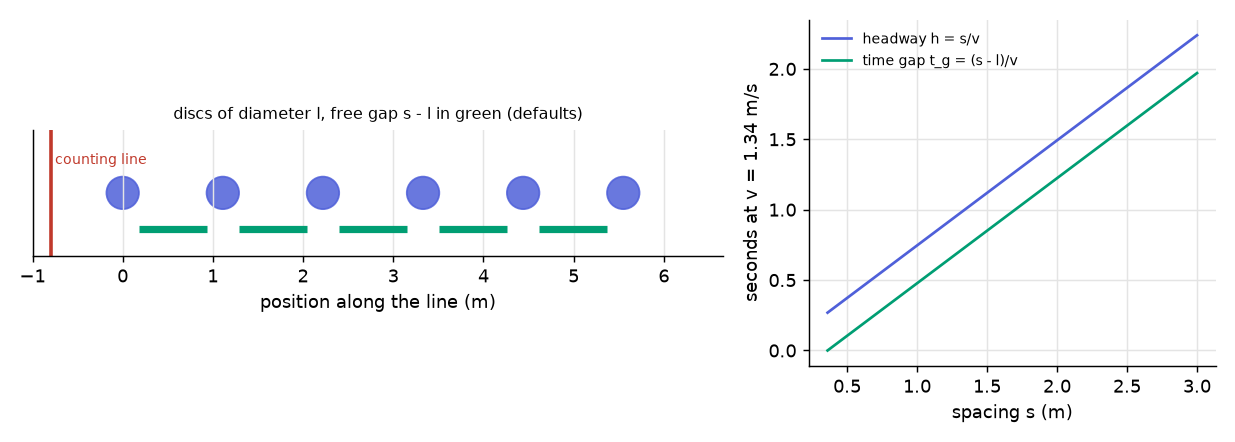
Concept check. A file has ρ = 0.9 ped/m and moves at 1.34 m/s. What is J, and what is the mean time between crossings? Answer: J = 0.9 × 1.34 = 1.206 ped/s; h = 1/J = 0.829 s.
2 · One rule per walker: the optimal-velocity function
The collision-free speed model sets a walker's speed from the spacing s ahead (tordeux2016_5e66 ↗):
Read it inside out. s − ℓ is the usable gap, because ℓ of the spacing is the body ahead. Dividing a length by T gives the speed that closes the gap in T seconds. max{0, ·} forbids walking backwards. min{v0, ·} caps the speed at the desired speed. In words: walk at your preferred speed unless that would leave less than T seconds of free gap to the person ahead.
The ramp has slope 1/T = 1.7857 s⁻¹ and starts at s = ℓ. It meets the plateau at the kink
Units: T·v0 is seconds times metres per second, so metres.
The three parameters, with units and a published value each:
| parameter | meaning | unit | value used | where it comes from |
|---|---|---|---|---|
| ℓ | pedestrian length (discs of diameter ℓ) | m | 0.36 | a in the required length d = a + b·v of Seyfried's single-file model (seyfried2006_f4db) |
| T | time gap | s | 0.56 | b in the same model, the value that agreed with the empirical single-file diagram (same paper) |
| v0 | desired speed | m/s | 1.34 | Weidmann's free speed, quoted in maury2018_d24a |
Three of the model's five parameters concern this function (tordeux2016_5e66 ↗). The corpus copy of that paper does not carry its parameter values (they sit in a figure that was not extracted), so the table takes ℓ and T from Seyfried's single-file model, whose required length d = a + b·v with a = 0.36 m and b = 0.56 s agreed with the empirical single-file diagram. On the congested branch the spacing equals the required length, so a plays the role of ℓ and b the role of T. Measured desired speeds are spread, not single-valued: a Gaussian with mean 1.30 m/s and standard deviation 0.21 m/s is quoted from Klüpfel et al., and 1.29 and 0.19 from Moussaïd et al. (maury2018_d24a ↗; wu2022_7ccd ↗). A group of 42 participants had a free speed of 1.55 ± 0.18 m/s (zhang2012_ab8c ↗). One number for v0 is already a choice.
Worked numbers at s = 0.80 m: usable gap 0.44 m, V = 0.44/0.56 = 0.7857 m/s, on the time-gap branch. V(ℓ) = 0, V(s*) = 1.34, V(1.5) = 1.34.
Break it: remove the clamp and set s = 0.30 m. V = (0.30 − 0.36)/0.56 = −0.1071 m/s, so the follower walks backwards. That is why max{0, ·} is in the rule.
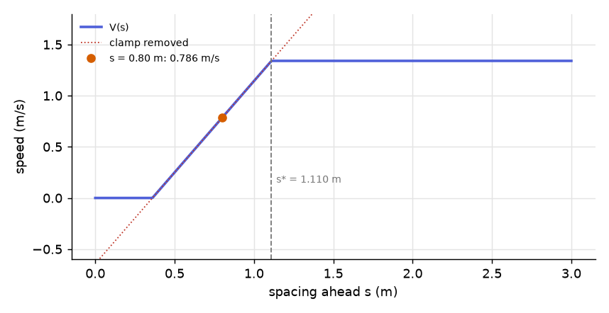
Concept check. Which branch is a walker on at s = 0.36 m, s = 0.8 m and s = 2 m? Answer: standstill (V = 0), time gap (V = 0.786 m/s), free (V = 1.34 m/s).
3 · From rule to law: the closed-form diagram and its capacity
Derivation. Assume a steady state of identical walkers with equal spacings. Then ρ = 1/s, and every walker follows V at that common spacing:
In words: at low density the crowd walks at the desired speed; past a critical crowding it walks as fast as keeps the time gap.
Free branch: J = v0·ρ, a line of slope v0. Congested branch:
linear in ρ with slope −ℓ/T = −0.6429 m/s (a speed, as a flow-per-density slope must be). The two branches meet where v0 = (1/ρ − ℓ)/T:
Consistency check: the congested branch at ρc gives (1 − ℓρc)/T = 1.2068 as well. The jam is where the congested speed reaches zero:
In words: below one walker per 1.11 m nobody is held up; above it every extra body carries flow but steals usable gap from the one behind, so throughput falls. The jam depends on body length only.
Per metre of width. Dividing by a lane width b converts ped/s into ped/(s·m). We take b = 0.60 m as an assumption (labelled so in the deck), giving J*/b = 2.011 ped/(s·m). With b = 0.45 m it is 2.682 and with b = 0.80 m it is 1.509. Door measurements typically sit at 2 to 3.5 ped/(s·m) (maury2018_d24a ↗, §9.5 to 9.6), which is 1.2 to 2.1 ped/s over a 0.60 m lane. The single-file capacity lands inside that band only under the assumed b.
The smooth cousin. The Weidmann spacing form with the same three parameters is
It has the same slope 1/T at s = ℓ and approaches the same plateau, and because 1 − e^{−x} ≤ x it lies below the OV rule everywhere. The largest gap is v0/e = 0.4929 m/s, at the kink s*, where v_W = 0.8470 m/s against 1.34. Its capacity is 0.7689 ped/s at ρ = 1.0078 ped/m, which is 0.637 of the triangle apex. The triangle overstates capacity because it lets everyone walk at full speed up to the apex, while a smooth law has already slowed them.
The areal Weidmann formula of section 7 maps onto this form by reading 1/ρ as area per person: ℓ ↔ 1/5.4 = 0.1852 m² and v0·T ↔ 1/1.913 = 0.5227 m². The exact equation of the spacing form is the standard one, consistent with the areal formula under s ↔ 1/ρ. The corpus copy of tordeux2019_877c ↗ confirms the parameter set (T, v0, ℓ) but its extracted text lost the equation, so the form is stated here as the standard one and not quoted.
A Weidmann-type fit to measured single-file data, v(w) = U(1 − e^{−(w − wm)/ws}) with U = 1.26 m/s, wm = 0.31 m and ws = 0.93 m, is reported in maury2018_d24a ↗. Written in the same form it has T = ws/U = 0.7381 s, and its peak is 0.6602 ped/s at 1.0218 ped/m.
Break it, twice. (a) Let T → 0. Then J* → v0/ℓ = 3.7222 ped/s, or 6.204 ped/(s·m) over 0.60 m, above the whole measured door band. At T = 0.05 s it is already 5.230 ped/(s·m). At the slider floor T = 0.3 s the capacity is 1.7585 ped/s = 2.931 ped/(s·m), still inside the band, which is why the deck has a separate "limit T → 0" button. (b) Set ℓ = 0.30 m: ρjam = 3.3333 ped/m, ρc = 0.9520 and J* = 1.2757 ped/s, while T and v0 have no say in ρjam. That one-line fact is why shrinking ℓ always clears a jam on paper. It is a geometry cheat, and Week 7 deals with it.
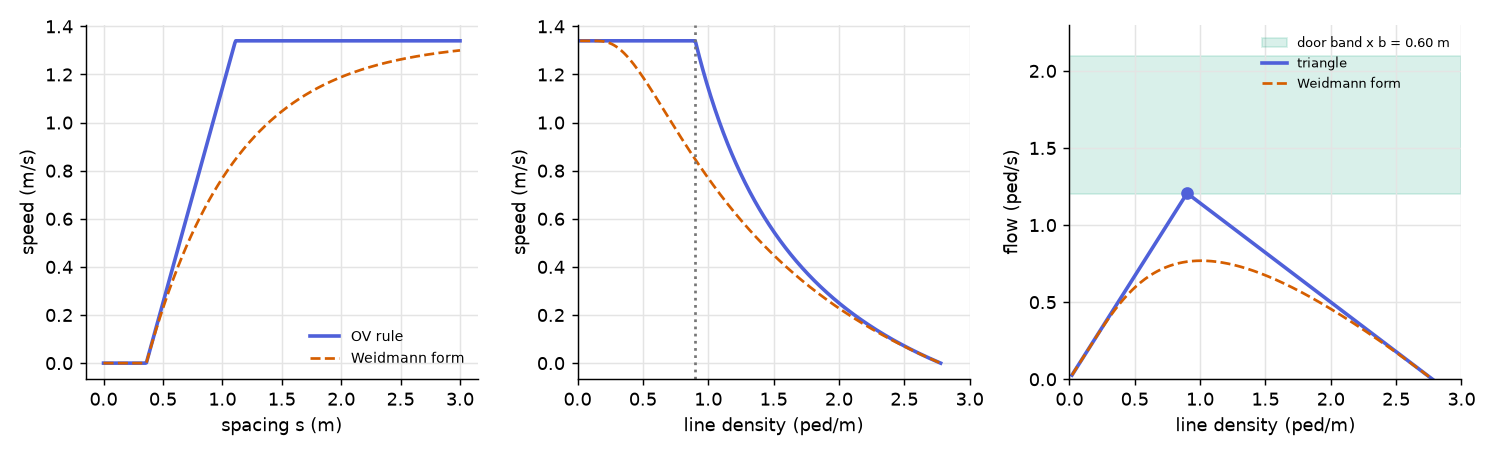
Concept check. With ℓ = 0.36 m and v0 = 1.34 m/s, why does J* fall when T rises? Answer: ρc = 1/(ℓ + T v0) falls and J* = v0 ρc falls with it: larger headway means fewer bodies per metre at the point where free flow ends. At T = 1.5 s, J* = 0.5654 ped/s.
4 · Does a crowd of rules obey the law? A single-file ring
The closed form assumed identical walkers in a settled state. To test it we put n walkers on a closed single-file ring of length L = 17.3 m, the system length used in Seyfried's single-file simulations (seyfried2006_f4db ↗). The update is explicit Euler, x_i ← x_i + dt·V(s_i), with dt = 0.05 s, for 300 s; the first half is discarded. Each walker has its own desired speed from N(1.34, 0.19²), clamped below at 0.3 m/s. The generator is mulberry32 with Box-Muller, ported bit for bit between the deck and the workbook. A pool of 45 draws is made once (mean 1.3597, sd 0.1966, min 0.8656, max 1.6908), and a run with n walkers uses the first n. Seyfried's own runs used desired speeds N(1.24, 0.05²) m/s, a much narrower spread, so this ring borrows his geometry and parameters but not his speed distribution.
Two results.
Congested branch: bookkeeping. When every walker is on the ramp, the mean speed is (L/n − ℓ)/T whatever the spacing distribution, because the gaps around a ring sum to L. At n = 40 the simulation gives 0.1295 m/s and the formula 0.1295 m/s. Agreement here is not evidence for the rule; it follows from arithmetic.
Free branch: the slowest walker. With no overtaking, every faster walker ends behind the slowest, so the system speed is min_i v0,i and not the mean:
In words: on a road nobody can overtake on, the slowest walker is the speed limit. The simulation matches this law at all 13 densities to better than 10⁻⁶ m/s. For n = 8 to 18 the speed is 1.0192 m/s, the smallest of the first n draws, while the homogeneous law with a common v0 = 1.34 gives 1.34 for n ≤ 15. At the default n = 18 (ρ = 1.0405 ped/m): simulated 1.0192, law 1.0192, homogeneous law 1.0734 m/s, 0 overlap events. Clones (σ = 0) hide all this: n = 10 gives exactly 1.3400 and n = 18 gives 1.0734. Other pools: seed 8 gives 0.9336 and seed 9 gives 0.9743 m/s at n = 18 (jitter seed fixed), and σ = 0.30 gives 0.8335.
The platoon gate is partly an artefact of a no-overtaking ring; in a real corridor faster walkers pass. What survives is the statement that a system's free speed is set by its constraints, not by the average preference. That agreement is also internal consistency: the simulation is the rule, so it cannot validate it.
Numerics: the time step. The continuous model is collision-free by construction, in the sense of an invariant set (tordeux2016_5e66 ↗); that paper's simulations use dt = 0.01 s. The Euler scheme is not collision-free for every dt. If the leader stands, the follower on the ramp moves dt·(s − ℓ)/T and its next gap is
which is below ℓ exactly when dt > T. Example, s = 1.0 m: dt = 0.30 s gives 0.6571 m, dt = 0.56 s gives 0.3600 m, dt = 0.70 s gives 0.2000 m, an overlap of 0.16 m. This condition is our derivation; the corpus states only that the update time in time-continuous models should be small enough that results do not depend on it (unknown2023_b047 ↗, the chapter on single-file dynamics).
Break it, n = 30 (ρ = 1.7341 ped/m, law 0.3869 m/s):
| dt (s) | overlap events | mean speed (m/s) | minimum gap (m) |
|---|---|---|---|
| 0.05 | 0 | 0.3869 | 0.5424 |
| 0.56 | 0 | 0.3869 | 0.5369 |
| 0.60 | 7959 | 0.4073 | 0.3005 |
| 0.80 | 231 | 1.0240 | 0.0166 |
| 1.00 | 42 | 1.2062 | 0.0056 |
At dt = 0.80 s the run reports about 1.02 m/s at a density where the law allows 0.387 m/s. A mean speed from a run with overlaps measures the scheme, not the law.
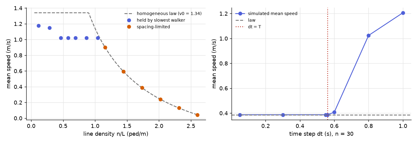
Concept check. Why does adding walkers to the pool never raise the plateau? Answer: the plateau is min_i v0,i over the walkers present; adding a walker can only keep or lower a minimum.
5 · Reading data backwards: the spacing-speed fit
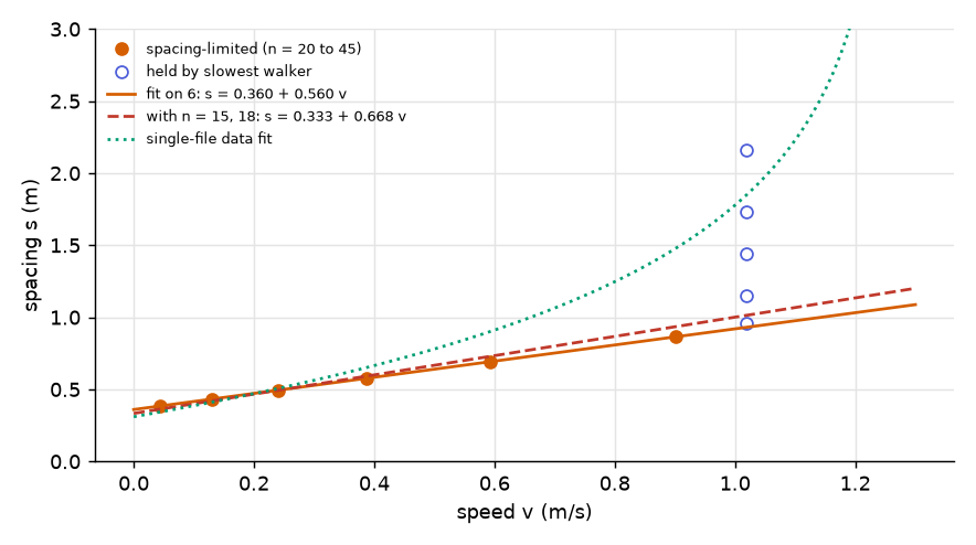
Empirical single-file work runs the road in reverse. On the congested branch s = ℓ + T·v, so a least-squares line of spacing on speed has the body length as intercept and the time gap as slope.
In words: the intercept is how much line a stopped person takes; the slope is how many seconds of headway each extra metre per second costs.
Seyfried's single-file model agrees with the empirical diagram with a = 0.36 m and b = 0.56 s, and does not with b = 1.06 s (seyfried2006_f4db ↗).
On the six spacing-limited ring runs (n = 20 to 45) the fit returns ℓ̂ = 0.3600 m and T̂ = 0.5600 s, the inputs, as it must in a simulation. The method is what matters, because point selection changes the answer. The runs at n = 15 and 18 look congested but are held by the slowest walker: at n = 15 the point is (v, s) = (1.0192 m/s, 1.1533 m), where the congested line would predict 1.4167 m/s. Including n = 15 and 18 gives s = 0.3333 + 0.6677·v, a slope 19.2% steeper from the same walkers. Noise is a smaller problem than selection: uniform ±0.05 m noise on s (seeded) gives s = 0.3781 + 0.5402·v, and ±0.10 m gives 0.3961 + 0.5204·v, from the six clean points.
A Weidmann-type single-file fit is not a straight line in this plane: with wm = 0.31 m it gives s = 0.7802 m at v = 0.5 m/s, against 0.64 m for the line s = 0.36 + 0.56·v. Over the range of the ring runs the two are not interchangeable.
Concept check. A single-file experiment yields s = 0.42 + 0.75·v. What are ℓ, T, ρjam? Answer: ℓ = 0.42 m, T = 0.75 s, ρjam = 1/0.42 = 2.381 ped/m.
6 · One knob, several literatures: the time-gap fan
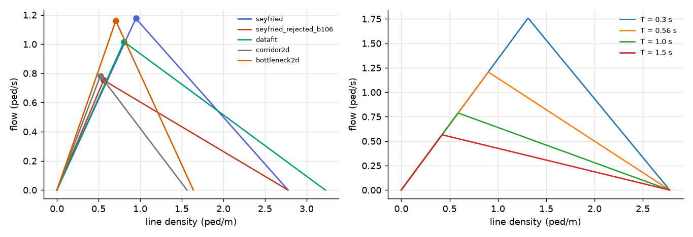
In a fixed-ℓ family the jam density is pinned by body length and the capacity fans out with T. With ℓ = 0.36 m and v0 = 1.34 m/s:
| T (s) | ρc (ped/m) | ρjam (ped/m) | J* (ped/s) |
|---|---|---|---|
| 0.30 | 1.3123 | 2.7778 | 1.7585 |
| 0.56 | 0.9006 | 2.7778 | 1.2068 |
| 1.00 | 0.5882 | 2.7778 | 0.7882 |
| 1.50 | 0.4219 | 2.7778 | 0.5654 |
J* falls by a factor 3.11 across the slider range while ρjam does not move. In words: body size decides where the crowd stops; headway decides how much it can carry. A capacity quoted without its T is not a number.
Published parameter sets, each as (ℓ, T, v0), with the triangle they imply:
| set | ℓ (m) | T (s) | v0 (m/s) | ρc | ρjam | J* (ped/s) |
|---|---|---|---|---|---|---|
| Seyfried single-file model | 0.36 | 0.56 | 1.24 | 0.9484 | 2.7778 | 1.1760 |
| Seyfried, rejected value b = 1.06 (v0 = 1.34 as elsewhere) | 0.36 | 1.06 | 1.34 | 0.5617 | 2.7778 | 0.7526 |
| single-file data fit (T = ws/U) | 0.31 | 0.7381 | 1.26 | 0.8065 | 3.2258 | 1.0161 |
| two-dimensional corridor | 0.64 | 0.85 | 1.50 | 0.5222 | 1.5625 | 0.7833 |
| two-dimensional bottleneck | 0.61 | 0.49 | 1.64 | 0.7074 | 1.6393 | 1.1602 |
Sources: seyfried2006_f4db ↗ for the first two rows, maury2018_d24a ↗ for the data fit, tordeux2019_877c ↗ for the last two. The same Weidmann-type model fitted to one population gives T ≈ 0.85 s in a corridor and 0.49 s at a bottleneck, with a higher desired speed at the bottleneck. The bottleneck set carries 1.48 times the corridor set's capacity.
Caveat. The two-dimensional fits use the mean distance to the ten nearest neighbours as the spacing, so their ℓ (0.64 and 0.61 m) is not a single-file body length. It lies outside the ℓ range 0.30 to 0.50 m of the widgets, which is why the deck shows them as fixed preset curves, not slider positions. The data-fit row is a triangle built from the fit's parameters, not the fitted curve itself.
Concept check. Why can two published capacities differ by a factor of 1.5 without either being wrong? Answer: they carry different T (and v0, ℓ) for behavioural reasons, and J* = v0/(ℓ + T v0) depends on all three.
7 · From files to floors, and where the law ends
Week 1's areal density returns. The jump: line density ρ (ped/m) becomes ρ in ped/m², and flow per file becomes specific flow Js in ped/(m·s), flow per metre of width. Weidmann's empirical relation, quoted in maury2018_d24a ↗ (§9.4), is
It was obtained by fitting 25 survey datasets (wu2022_7ccd ↗). The primary handbook is not in the corpus; the formula reaches this course through secondary sources.
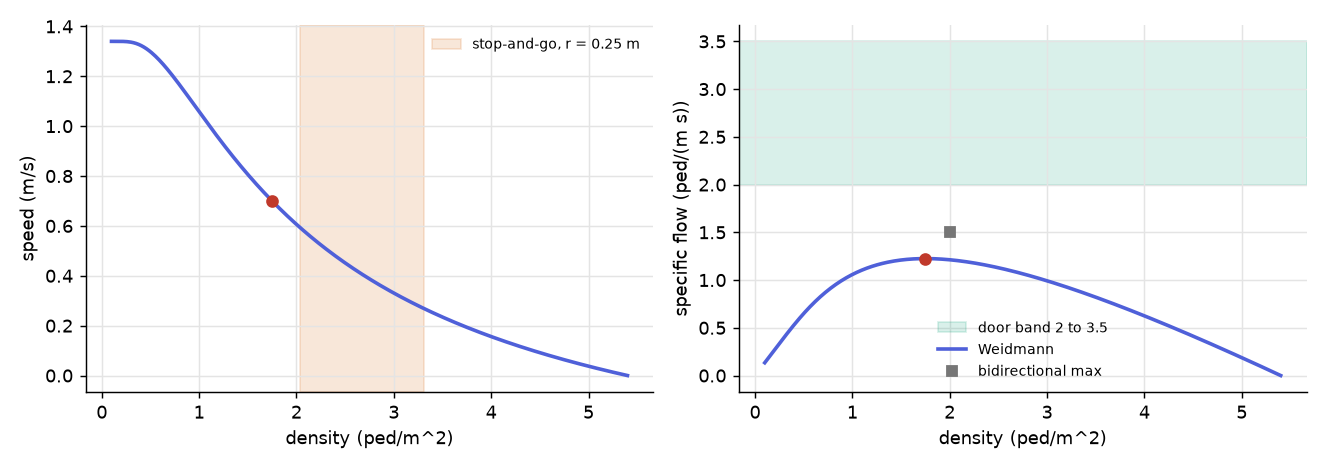
Worked numbers at ρ = 1.75 ped/m²: v = 0.7000 m/s, Js = 1.2249 ped/(m·s). The maximum is Js = 1.2249 at ρ = 1.7507 (v = 0.6997 m/s). Speeds at ρ = 0.5, 1, 2, 3, 4, 5 are 1.2984, 1.0581, 0.6062, 0.3307, 0.1563 and 0.0374 m/s. In words: a corridor of strangers moves the most people per metre of width at under two per square metre.
One curve per facility. Door measurements sit at 2 to 3.5 ped/(s·m), 1.6 to 2.9 times the Weidmann maximum: about 3.5 at 220 cm width and lower at other widths (Daamen et al.), with a capacity drop of 18 to 28% at a 90 cm restriction and about 15% at 60 cm (Cepolina), all quoted in maury2018_d24a ↗ and used here only as comparison values. Bidirectional corridor flow has a specific-flow maximum of 1.5 ped/(m·s) at 2.0 ped/m² (zhang2012_ab8c ↗), against 1.2125 from the Weidmann formula at 2.0. These are different facilities with different behaviour, not one law with noise. The single-file capacity of section 3 is 2.011 ped/(s·m) only under the assumed b = 0.60 m.
Why a peak exists. The flux maximum is connected to intra- and interpersonal variability of walking speeds; with identical constant speeds the flux would grow linearly up to capacity (corbetta2023_bcb7 ↗).
Where the law ends. Above the formula's domain the speed goes negative: v = −0.0483 m/s at ρ = 6.0, which is not a prediction of anything. Earlier still, an equation-of-state picture fails. A behavioural model shows stop-and-go waves at 40 to 65% spatial coverage, with backward waves near 0.6 m/s, and above that crowd turbulence, where physical forces replace intentional motion and the displacement statistics follow a power law with exponent 1.95 ± 0.09 (moussad2011_fa42 ↗); an observed exponent of 2.01 is reported in helbing2015_d0b0 ↗, which describes a global breakdown of coordination. Occupancy is φ = ρπr². The model of moussad2011_fa42 ↗ uses r = m/320 with masses of 60 to 100 kg, that is r ≈ 0.19 to 0.31 m; at r = 0.25 m (an assumption in the deck) the stop-and-go band is ρ = 2.04 to 3.31 ped/m², and at r = 0.20 m it is 3.18 to 5.17. At ρ = 1.75 and r = 0.25 m, φ = 0.344. The band starts at 2.04 ped/m², well before the formula's own jam at 5.4. Where no v(ρ) exists, a law of the form v(ρ) is not a valid description at all.
Concept check. A designer applies the Weidmann formula at ρ = 4 ped/m². What does it return and what should she worry about? Answer: v = 0.1563 m/s, Js = 0.625 ped/(m·s). At r = 0.25 m that density is φ = 0.79, above the 40 to 65% stop-and-go band, so the formula is being used where a speed-density law is not expected to hold.
Exam questions
Q1 · Derivation. Starting from V(s) = min{v0, max{0, (s − ℓ)/T}}, derive the single-file fundamental diagram and show that J(ρ) is a triangle with apex at ρc = 1/(ℓ + T·v0). Model answer. Assume equal constant spacings, so ρ = 1/s and v(ρ) = min{v0, (1/ρ − ℓ)/T}. Free branch: J = v0ρ, rising. Congested branch: J = ρ(1/ρ − ℓ)/T = (1 − ℓρ)/T, linear, slope −ℓ/T (units m/s), zero at ρjam = 1/ℓ. J rises on one side of the branch point and falls on the other, so the maximum is at the branch point; equating v0 = (1/ρ − ℓ)/T gives ρc = 1/(ℓ + T v0) and J* = v0/(ℓ + T v0). Both branches give the same J* at ρc.
Q2 · Inverse problem. A single-file experiment yields s = 0.42 + 0.75·v (metres, seconds). Take v0 = 1.34 m/s. Give ℓ, T, ρjam, ρc, J*. Model answer. ℓ = 0.42 m, T = 0.75 s. ρjam = 1/0.42 = 2.381 ped/m. ρc = 1/(0.42 + 0.75 × 1.34) = 1/1.425 = 0.702 ped/m. J* = 1.34 × 0.7018 = 0.940 ped/s = 56.4 ped/min. ℓ is anatomy and T is behaviour; ρjam depends on ℓ only.
Q3 · Heterogeneity. Why do per-walker desired speeds matter on a no-overtaking ring, and what limits the argument? Model answer. Each walker's v0 is drawn from a distribution; on the free branch every faster walker ends behind the slowest, so the system speed is min_i v0,i (1.0192 m/s for n = 18 in the executed run), not the mean or the common 1.34. Clones give 1.34 (n = 10) and hide the effect. On the congested branch the mean speed is (L/n − ℓ)/T regardless, because gaps sum to L, so agreement there is bookkeeping. The limit: the gate is partly a no-overtaking artefact; a corridor with overtaking lets faster walkers pass.
Q4 · Validity. "With a good fundamental diagram we can model crowd behaviour at any density." Refute in one paragraph. Model answer. A speed-density law is an equation-of-state relation. It requires that behaviour is a function of density. Weidmann's formula is undefined past 5.4 ped/m² (returns v < 0 at 6.0). Before that, behavioural models show stop-and-go waves at 40 to 65% coverage and, above that, crowd turbulence with power-law displacement statistics (exponent about 1.95 to 2.01), where physical forces replace intentional motion (moussad2011_fa42 ↗; helbing2015_d0b0 ↗). No v(ρ) describes that regime.
Q5 · Time step. A ring simulation at n = 30 reports a mean speed of 1.02 m/s at dt = 0.80 s and 0.387 m/s at dt = 0.05 s, both with T = 0.56 s, ℓ = 0.36 m. Explain, and state the rule for choosing dt. Model answer. With a standing leader the follower's next gap is ℓ + (s − ℓ)(1 − dt/T); for dt > T this is below ℓ: bodies overlap, V clamps to zero, and the following step jumps. The run at 0.80 s logs 231 overlap events and its mean speed is not a measurement of the law, which predicts 0.387 m/s. Choose dt ≤ T at minimum, and small enough that results no longer depend on it.
Q6 · Capacity without its parameters. A report states "single-file capacity is 1.2 ped/s" and another "0.78 ped/s" for corridors. Can both be right? Model answer. Yes: J* = v0/(ℓ + T v0) depends on all three parameters. With ℓ = 0.36, T = 0.56, v0 = 1.34, J* = 1.2068; with T = 1.06 it is 0.7526, and a corridor set with ℓ = 0.64, T = 0.85, v0 = 1.50 gives 0.7833. A capacity quoted without (ℓ, T, v0), and without the facility, is not a number. Per metre of width it also needs a stated lane width.
Where this goes next
The fundamental diagram is the first test a force model must pass (Week 3), and per-walker desired speeds carry over. The collision-free property holds in continuous time only (section 4), and the two-dimensional spacing caveat of section 6 motivates the side-by-side corridor (Week 4). J(ρ) from sections 3 and 7 is the flux the conservation law uses in Week 5. The spacing-speed fit and its selection bias set up the method trap of Week 6. The door band and the capacity drop return in Week 8.
Further reading
- tordeux2016_5e66 ↗: the optimal-velocity function, its parameters and the collision-free property.
- seyfried2006_f4db ↗: the single-file model on a ring of 17.3 m, a = 0.36 m and b = 0.56 s.
- tordeux2019_877c ↗: Weidmann-type fits in a corridor and at a bottleneck.
- maury2018_d24a ↗: the areal Weidmann formula, the single-file data fit, desired-speed statistics and door capacities.
- corbetta2023_bcb7 ↗: why the flux maximum exists.
- wu2022_7ccd ↗: the 25-survey provenance of Weidmann's relation, and a Gaussian desired-speed fit.
- zhang2012_ab8c ↗: bidirectional specific flow and a free-speed sample.
- moussad2011_fa42 ↗: stop-and-go waves and crowd turbulence.
- helbing2015_d0b0 ↗: crowd turbulence and the limits of equilibrium descriptions.
- unknown2023_b047 ↗: single-file dynamics and the update-time remark.
Provenance (instructor only)
Executed sources, vault paths:
- obsidian/monad-knowledge/edu/courses/CRD503-crowd-dynamics-simulation/week-02-the-fundamental-diagram/workbook.ipynb
- obsidian/monad-knowledge/edu/courses/CRD503-crowd-dynamics-simulation/week-02-the-fundamental-diagram/numbers.json
Literature notes (where each cited figure sits):
- literature/Collision-Free Speed Model for Pedestrian Dynamics.md (rule, parameter roles, collision-free property, dt = 0.01 s; parameter values absent from the extracted text)
- literature/Basics of modelling the pedestrian flow.md (Results: L = 17.3 m, N(1.24, 0.05) m/s, a = 0.36 m, b = 0.56 s and 1.06 s)
- literature/Artificial Neural Networks Predicting Pedestrian Dynamics in Complex Buildings.md (Speed-Based Model, Data Analysis: T, v0, ℓ, K = 10 neighbours; equation not in the extracted text)
- literature/Crowds in Equations.md (§9.4 Weidmann formula and single-file fit, book p.150; desired speeds, book p.149; §9.5 to 9.6 door capacities, book p.151)
- literature/Physics of Human Crowds.md (flux maximum and speed variability)
- literature/An Extended Social Force Model via Pedestrian Heterogeneity Affecting the Self-Driven Force.md (Moussaïd desired speeds; 25 survey datasets)
- literature/Ordering in bidirectional pedestrian flows and its influence on the fundamental diagram.md (free velocity of 42 participants; bidirectional specific-flow maximum)
- literature/How simple rules determine pedestrian behavior and crowd disasters.md (Results and Model: 40 to 65% coverage, 0.6 m/s waves, exponent 1.95 ± 0.09, r = m/320)
- literature/Saving Human Lives What Complexity Science and Information Systems can Contribute.md (crowd turbulence, exponent 2.01)
- literature/Crowd Dynamics, Volume 4.md (single-file chapter, §5.3, update time)
Corpus silences and derivations:
- No primary Weidmann handbook, no primary Greenshields paper, and no primary Seyfried 2005 or Jelić 2012 single-file paper are in the corpus; they are reached only through the notes above.
- The Euler condition dt ≤ T for the first-order rule has no corpus source; it is derived in section 4.
- The 0.60 m lane width and the body radius 0.25 m are assumptions, labelled as such in the deck.
- The corpus dictionary has no entry for time gap, stop-and-go waves or crowd turbulence.
- "Bidirectional flow is lower" compares with the door band (1.5 against 2 to 3.5 ped/(s·m)); against the areal Weidmann maximum (1.2249) the bidirectional maximum is higher.