Companion to the deck. The deck is the primary material: every idea below is a live widget there, and the numbers printed here are the numbers those widgets show at their default state. The workbook (workbook.ipynb) computes every one of them; numbers.json holds the same list.
Week 1 gave the continuous channel H(f) = \sum_i a_i e^{-j 2\pi f \tau_i}. This week samples that function at a row of tones, shows how a receiver measures each sample, and shows how three radios lay the samples out in memory.
Conventions used throughout: the direct path is normalised to 1, tones sit at f_k = f_c + k\,\Delta f, and the standard test channel is two paths, H_k = 1 + a\,e^{-j 2\pi f_k \tau}, on the 52 used legacy tones (k = -26..-1, 1..26, spacing 312.5 kHz).
1. Why CSI and not RSSI
Idea. RSSI is 10\log_{10} of the total received power. It is one real number per packet. Many different channels have the same total power, so RSSI cannot tell them apart. CSI keeps one complex number per tone.
Derivation. For the two-path channel the power averaged over the 52 tones is
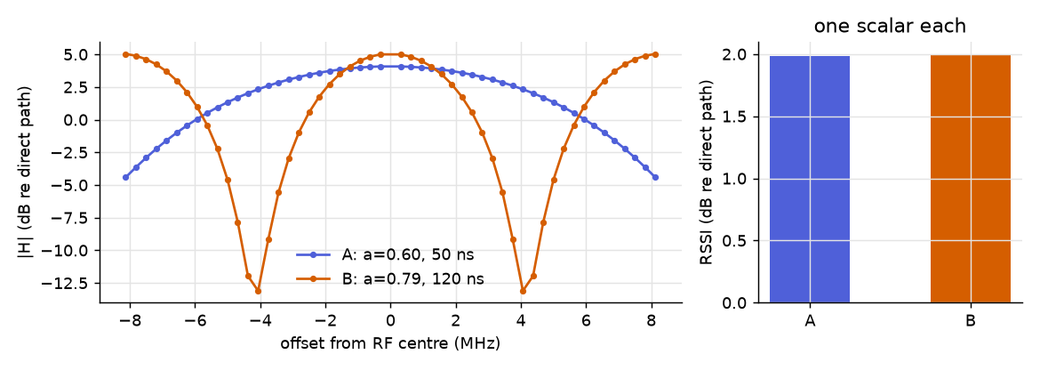
Fix a channel A (a = 0.60, τ = 50 ns). For any other delay τ there is an amplitude a_B that solves 1 + a_B^2 + 2 a_B \bar c(\tau) = P_A, so a whole family of channels shares A's RSSI.
In words: the power sums the squared lengths of the tone vectors and forgets which tone was long and which was short. Any channel that redistributes power across tones without changing the total is invisible to RSSI.
Worked numbers (workbook section 1). Channel A has RSSI 1.983 dB relative to the direct path. Channel B (τ = 120 ns) with the exact matching amplitude 0.7868 has RSSI 1.983 dB. At the slider value a_B = 0.79 the RSSI is 1.9964 dB, a difference of 0.0133 dB. The per-tone curves differ strongly: A ranges from -4.41 to +4.07 dB across the tones, B from -13.10 to +5.03 dB, and the largest single-tone gap is 15.43 dB. The Euclidean distance between the two 52-value CSI vectors is 7.66, which is 0.846 of the length of A's vector. Of the 21 delays from 0 to 200 ns in 10 ns steps, 19 admit an equal-RSSI partner with amplitude at most 1.
Concept check. Given only RSSI, can you recover the echo delay? No: every delay in the family above produces the same RSSI. What extra information does the per-tone vector carry that pins the delay down? The rate at which |H_k| ripples across tones.
2. OFDM is a comb of tones
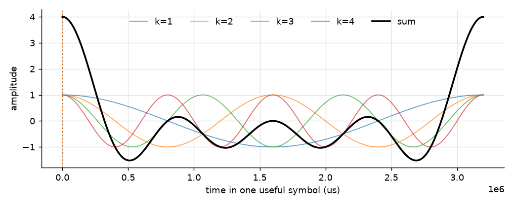
Idea. OFDM transmits many narrow tones at once. One antenna sends their sum. Tones are spaced \Delta f apart and one useful symbol lasts T_u = 1/\Delta f, so every tone completes a whole number of cycles inside the symbol.
Derivation.
Two tones m \ne k satisfy \frac{1}{T_u}\int_0^{T_u} e^{j2\pi(m-k)\Delta f t}\,dt = 0, so a receiver can read each X_k out of the sum without interference from its neighbours. The fast way to evaluate the sum on N samples is the inverse FFT.
In words: each tone is a sinusoid that fits an integer number of times into the symbol, and integer-cycle sinusoids do not leak into each other.
Worked numbers (workbook section 2). T_u is 3.2 µs at 312.5 kHz and 12.8 µs at 78.125 kHz. Tone k always completes k cycles per useful symbol; tone k = 2 at 312.5 kHz sits at 0.625 MHz with period 1.6 µs. With tones 1 to 4 all in phase, x at 0.6 µs is -1.2483, the sum of the terms 0.3827, -0.7071, -0.9239 and 0.0. The numerical inner product of tones 1 and 2 over one symbol has magnitude 0.0; tone 2 with itself has magnitude 1.0. Detune tone 2 by half a cycle (2.5 cycles per symbol) and its overlap with tone 1 becomes 0.212 instead of 0, while its overlap with its own grid slot drops to 0.637: tones off the grid leak, which is why carrier frequency offset harms OFDM. An inverse FFT of size 64 reproduces the direct sum exactly and has a sample period of 50 ns at 20 MHz. In-phase tones add to a peak of 4.0 against a mean power that gives a peak-to-average power ratio of 9.03 dB, which is why real transmitters choose the tone phases with care. A guard interval of 0.8 µs makes the legacy symbol 4.0 µs, a guard fraction of 0.2.
Concept check. If the spacing drops to 78.125 kHz, how many cycles does tone 2 complete per useful symbol, and how long does that symbol last? Two cycles, 12.8 µs.
3. Estimating H from a known symbol
Idea. The receiver knows the training symbol X_k it should have received. Dividing what arrived by what was sent gives the channel at each tone, plus noise.
Derivation.
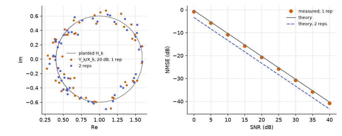
With unit-energy training and noise variance \sigma^2 = 10^{-\mathrm{SNR}/10} per tone, the mean squared error is \sigma^2, and averaging R repetitions of the training symbol divides it by R:
In words: the estimate is the truth plus scaled noise; more SNR or more repetitions shrink the noise, nothing else does.
Worked numbers (workbook section 3; planted channel 1 + 0.6e^{-j2\pi f_k \cdot 80\,\mathrm{ns}} with \overline{|H|^2} = 1.0861; training is a seeded ±1 stand-in sequence, seed 7). At 20 dB and one repetition the measured error is -20.80 dB against the formula's -20.36 dB. Over seeds 1 to 200 the measured value has mean -20.25 dB and standard deviation 0.58 dB, so the seed-7 value is an ordinary draw. Two repetitions give -23.22 dB measured against -23.37 dB from the formula (expected gain 3.01 dB). The SNR sweep with one repetition reads -0.80, -10.80, -20.80, -30.80 and -40.80 dB at 0, 10, 20, 30 and 40 dB; the noise draws are reused across SNR, so the points are exactly 10 dB apart. On tone k = 1 the planted value is 1.5926 - 0.0939j and the estimate is 1.5869 - 0.0557j.
Concept check. Why does doubling the repetitions gain 3 dB and not 6? Noise variance halves (3.01 dB), and error power is proportional to variance.
4. Vendor tone layouts
Idea. Three labels are easy to confuse: the array position i of a stored coefficient, the subcarrier index k it belongs to, and its frequency f = f_c + k\,\Delta f. A profile is the rule that maps i to k.
| Profile | Entries | Spacing | T_u | k range | Edge offset | Word size | FFT |
|---|---|---|---|---|---|---|---|
| AX210 legacy20 | 52 | 312.5 kHz | 3.2 µs | -26..-1, 1..26 | 8.125 MHz | 16 bit | 64 |
| AX210 HT20 | 56 | 312.5 kHz | 3.2 µs | -28..-1, 1..28 | 8.75 MHz | 16 bit | 64 |
| AX210 HE20 SU | 242 | 78.125 kHz | 12.8 µs | -122..-2, 2..122 | 9.5312 MHz | 16 bit | 256 |
| ESP32-C5 legacy L-LTF | 53 | 312.5 kHz | 3.2 µs | SDK order 0..26, -26..-1 | 8.125 MHz | 8 bit | 64 |
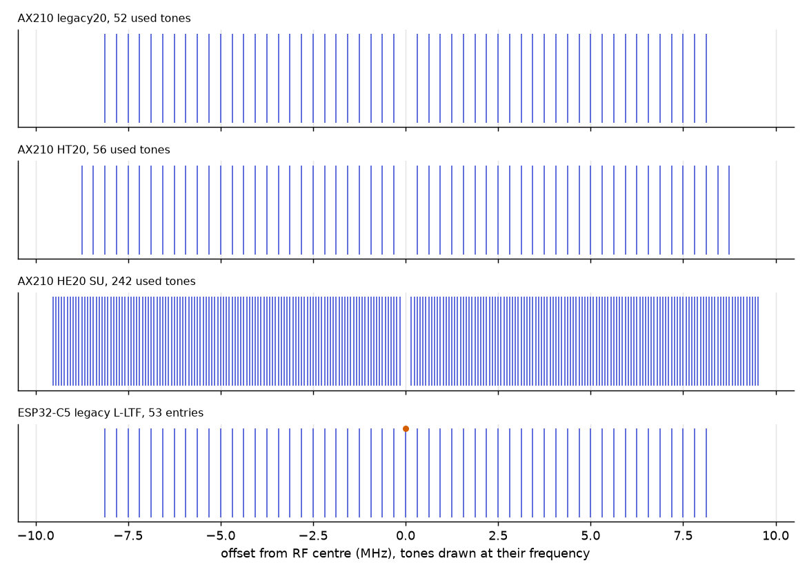
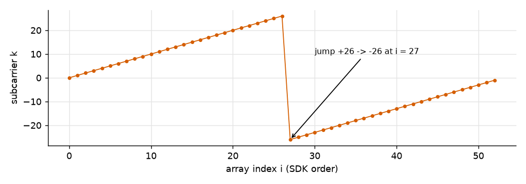
Derivation. The mapping is a table lookup, not arithmetic: k = \mathrm{tones}[i]. Legacy and HT store negative tones first, then positive, and omit k = 0. HE20 omits three tones, k = -1, 0, +1. The C5 buffer keeps DC first: index 0 is k = 0, indices 1 to 26 are k = 1..26, indices 27 to 52 are k = -26..-1, and the DC entry holds a null.
In words: the array is a storage order; the frequency axis is a different order. Plotting one against the other without the table draws a false spectrum.
Worked numbers (workbook section 4, RF centre taken as 5200 MHz for the examples). AX210 legacy20 at i = 30 gives k = 5, offset +1.5625 MHz, absolute 5201.5625 MHz; the first positive tone is at i = 26 and the missing DC tone leaves a 625 kHz gap between the last negative and the first positive entry. HT20 at i = 0 gives k = -28, offset -8.75 MHz. HE20 stores k = -2 at i = 120 and k = +2 at i = 121; the three-tone hole is 312.5 kHz wide between neighbours, and i = 121 sits at +0.15625 MHz, absolute 5200.15625 MHz. In ESP32-C5 array order, i = 26 is k = +26 (5208.125 MHz) and i = 27 is k = -26 (5191.875 MHz): an apparent jump of -16.25 MHz between adjacent array positions, a false band edge. One C5 block is 106 bytes (53 pairs of 8-bit words); one AX210 legacy20 chain is 208 bytes.
Concept check. A sorted-by-frequency plot of the C5 buffer versus a plot in array order: which one has a discontinuity in the middle? The array-order plot; the sorted plot puts the DC null at the centre.
5. CFR and CIR are a DFT pair
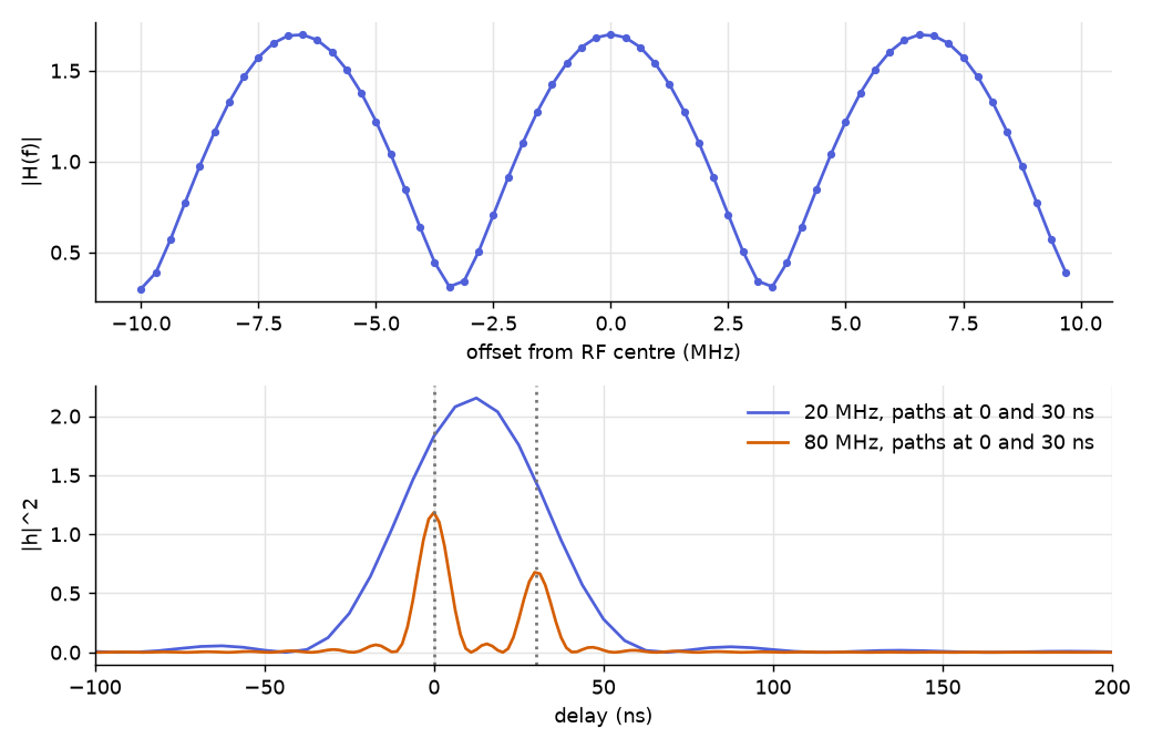
Idea. The per-tone response (CFR) and the delay-domain response (CIR) are one channel in two views, related by a DFT. Two numbers control what the CIR can show: the bandwidth B sets the delay resolution, and the tone spacing \Delta f sets the largest delay that is not aliased.
Derivation. With N contiguous tones at spacing \Delta f, B = N\Delta f and the CIR sample spacing is 1/B:
Two paths closer than \Delta\tau fall inside one CIR bin and merge. Padding the DFT with zeros interpolates the curve between bins; it adds no tones and therefore no resolution. A window trades width for side lobes: Hann widens the main lobe and suppresses the side lobes.
In words: bandwidth is the length of the ruler in frequency, and a longer frequency ruler gives finer ticks in delay.
Worked numbers (workbook section 5).
| Bandwidth | Tones at 312.5 kHz | \Delta\tau | \Delta d |
|---|---|---|---|
| 20 MHz | 64 | 50 ns | 14.99 m |
| 40 MHz | 128 | 25 ns | 7.49 m |
| 80 MHz | 256 | 12.5 ns | 3.75 m |
| 160 MHz | 512 | 6.25 ns | 1.87 m |
The maximum unambiguous delay is 3200 ns (959.3 m) at 312.5 kHz and 12800 ns (3837.3 m) at 78.125 kHz; a path at 3300 ns would appear at 100 ns. For two paths at 0 and 150 ns (amplitudes 1 and 0.7) at 20 MHz, the rectangular window shows peaks at 0 and 137.5 ns with powers 1.0 and 0.506: the side lobe of the first path pulls the second peak by -12.5 ns. Under a Hann window the peaks sit at 0 and 150 ns with powers 0.997 and 0.487. A single path has a half-power width of 43.75 ns (rectangular) against 68.75 ns (Hann) and a highest side lobe of -13.26 dB against -31.50 dB. Break the method: place the second path 30 ns from the first. The profile shows one peak at 20 MHz and at 40 MHz, and two at 80 MHz and 160 MHz. At 20 MHz the peak count stays at one for padding factors 1, 4 and 8, and for the Hann window at both padding values.
Peak counting depends on the relative amplitude and the detection threshold (here 15 percent of the maximum), so 1/B is a rule of thumb, not a sharp limit; at 40 MHz (\Delta\tau = 25 ns) the two paths 30 ns apart still merge for these amplitudes.
Concept check. Zero padding to eight times the tones makes the 20 MHz curve look smooth. Does it separate the two paths 30 ns apart? No; the peak count remains one.
Literature. The resolution rule is stated in xie2015_0389 ↗: paths whose delays differ by less than 1/B are not distinguishable, and in a 20 or 40 MHz channel the path-length uncertainty is 15 m or 7.5 m. cominelli2023_e6ee ↗ states that a broader CSI bandwidth helps discriminate paths that arrive close to the first one, while higher spectral resolution helps detect multipath components with larger delays. gringoli2022_1c5c ↗ shows HE frames use a four times smaller spacing (78.125 kHz instead of 312.5 kHz), which is the second control in the formulas above.
6. The tensor the card hands you
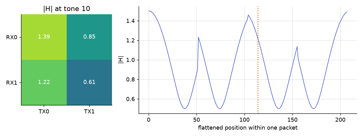
Idea. One packet yields one coefficient per receive chain, transmit stream and tone: H[\text{packet}, \text{rx}, \text{tx}, \text{tone}]. Storage flattens it. The convention used in this course is chain-major: \text{chain} = \text{rx}\cdot n_\text{tx} + \text{tx} and
In words: tones vary fastest, then transmit stream, then receive chain, then packet.
Worked numbers (workbook section 6; 2x2, K = 52, packet 2, rx 1, tx 0, tone index 10). Chain 2, 208 coefficients per packet, offset 530 (114 within packet 0). The illustrative coefficient there has magnitude 1.2187; the four spatial entries at tone 10 are 1.3865, 0.8466, 1.2187 and 0.6135 for (rx0,tx0), (rx0,tx1), (rx1,tx0), (rx1,tx1). That pattern is synthetic and carries no physical meaning.
The 2x2 grid of the widget is an abstract layout. The number of transmit streams in a record is the number the frame trains: a legacy (non-HT) frame trains one, so an AX210 legacy20 record is 2 receive chains by 1 stream. Size of a packet's coefficients with two 16-bit words per coefficient (4 bytes): AX210 2x1 legacy20 is 104 coefficients, 416 bytes (208 bytes per chain); 2x2 HE20 is 968 coefficients, 3872 bytes; 2x2 HE80 is 3984 coefficients, 15936 bytes. At 160 MHz an open-source Linux 802.11ax CSI tool reports a 1 x 2 x 1992 matrix on the AX210 (transmit antennas, receive antennas, subcarriers), 4 bytes per subcarrier plus a 272-byte header, 16208 bytes per measurement (zhang2025_72c4 ↗); the workbook reproduces 3984 coefficients, 15936 bytes, 16208 with the header. If two streams were trained at 160 MHz the packet would be 7968 coefficients, 31872 bytes, 3.19 MB/s at 100 packets/s. One C5 block (one chain, 53 8-bit pairs) is 106 bytes, so that hypothetical widest AX210 packet is about 300 times larger.
The ESP32-C5 has a single receive chain. The reporting bandwidth of the AX210 depends on the monitor width relative to the frame width: a 996-tone HE80 record appears only when the monitor width is at least the frame width. gringoli2022_1c5c ↗ documents, for a different 802.11ax chipset, that each spatial stream of a 160 MHz HE frame occupies up to 2048 subcarrier slots in the chipset's tables; 1992 of them are reported as used tones by the AX210 tool above.
Concept check. Give the offset of H[\text{packet}=1, \text{rx}=0, \text{tx}=1, \text{tone}=5] in a 2x2, K = 52 layout. 1\cdot 208 + (0\cdot 2 + 1)\cdot 52 + 5 = 265.
7. One coefficient: a point, a length and an angle
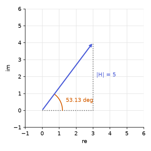
Idea. Two stored words become \text{re} + j\,\text{im}. Length and angle follow:
A null (0 + j0) has a length of 0 and no angle. The level is relative to one raw unit; a separate gain control on the card sets the scale, so the number is only comparable within one packet.
Worked numbers (workbook section 7; default 3 + j4). |H| = 5, angle 0.9273 rad = 53.13 degrees, level 13.98 dB (13.9794 dB) in raw units. Swap the two words: 4 + j3 has the same length 5 and the angle 36.87 degrees, an error of -16.26 degrees, so swapping I and Q corrupts phase and leaves amplitude intact. Word size sets the range: signed 8-bit words span -128..127 (dynamic range 42.08 dB), signed 16-bit words span up to 32767 (90.31 dB). Saturation distorts the angle: a true pair (200, 150) has angle 36.87 degrees, but clipped to 8 bits it becomes (127, 127) with angle 45.0 degrees and length 179.61.
Concept check. A decoder reads every coefficient with the words in the wrong order. Which of |H| and \angle H survives? |H| survives; \angle H becomes \pi/2 - \angle H.
8. Wider channels, more independent structure
Idea. Tone groups far apart in frequency see different combinations of the paths when the delay spread is large. A wide channel therefore has more groups that behave independently. The price is noise: the same transmit power spreads over more tones.
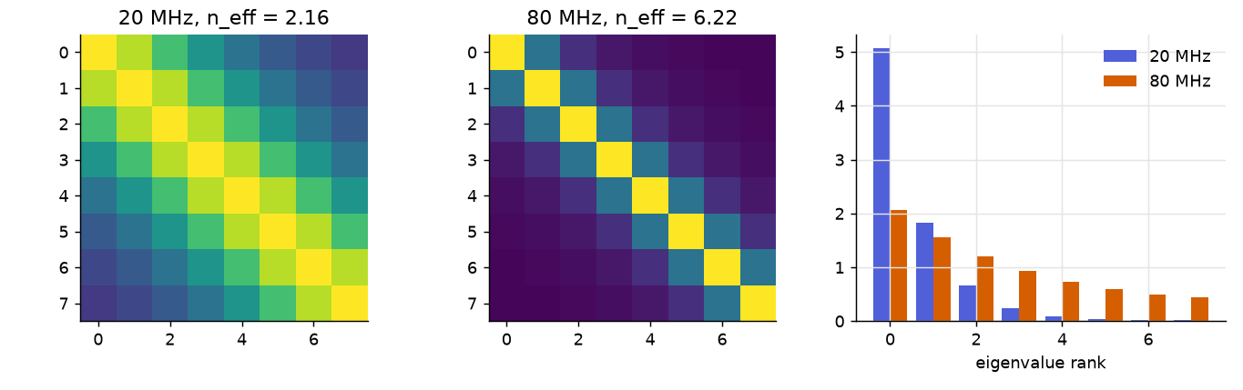
Derivation (the widget's model, qualitative). For an exponential power-delay profile with RMS spread \sigma_\tau, the complex correlation between tones d apart is \rho(d) = 1/(1 + j2\pi d\,\sigma_\tau) and the power correlation is |\rho|^2. Take eight tone groups spread evenly across the bandwidth, build the 8\times 8 matrix of |\rho|^2, shrink the off-diagonal terms by \left(\frac{s}{1+s}\right)^2 for per-tone SNR s (independent noise decorrelates groups) while the diagonal stays 1, and define
over the eigenvalues \lambda_i of that matrix (the participation ratio). It is 1 if one eigenvalue carries everything and 8 if all groups are independent.
In words: n_\text{eff} counts how many of the eight groups carry information that the others do not.
Worked numbers (workbook section 8; default \sigma_\tau = 20 ns, SNR 20 dB; the 20 ns value is a teaching assumption, not a measurement). At 20 MHz the groups are 2.5 MHz apart, adjacent correlation 0.8922, farthest 0.168, n_\text{eff} = 2.16. At 80 MHz the groups are 10 MHz apart, adjacent correlation 0.3801, farthest 0.0125, n_\text{eff} = 6.22. Break it: shrink the delay spread. At 5 ns, n_\text{eff} is 1.16 at 20 MHz and 2.16 at 80 MHz; at 10 ns it is 1.44 and 3.69; at 100 ns it is 6.93 and 7.99. The model has a caveat that matters for interpretation: lowering the SNR raises n_\text{eff} (at 0 dB SNR and 20 ns, 6.80 at 20 MHz), because independent noise looks like independent structure. A rise of n_\text{eff} alone therefore does not show that the channel changed; a control that holds the noise fixed is required. The noise penalty of the wider channel at equal transmit power is 10\log_{10}(80/20) = 6.02 dB per tone.
A measured contrast. One transmitter sent 200-byte frames at 100 frames per second on a 5 GHz channel in a library, to six receivers, each with two antennas. The transmitter ran in two modes: an 80 MHz VHT source and a 20 MHz legacy source (the frame format changed together with the width). For each receiver link the CSI of eight tone groups was reduced to a dynamic-power series and n_\text{eff} was computed by the same participation ratio as above. By day, in three time-of-day slots and at all six receivers, the mean n_\text{eff} was 1.89 for the 20 MHz source and 3.80 for the 80 MHz source, a mean paired difference of +1.95. At night the two widths gave the same value, 1.36. The quiet-link floor (5th percentile of the dynamic share of power) was about ten times higher for the 80 MHz source, 0.079 against 0.008. The result is a mechanism pilot with n = 3 slots and carries no significance claim; the night comparison used a single 20 MHz night block recorded on a different night from the 80 MHz blocks. The pattern is consistent with an extra frequency structure that appears with activity in the room and with a noise cost that is present at all times. The model above reproduces the direction of the day contrast, not the values, and the pilot cannot separate the effect of width from the effect of the frame format.
Concept check. Why is the night value informative? If the extra groups were only receiver noise they would also appear at night; at night the two widths agree, which argues against a pure noise explanation.
Key numbers
| Quantity | Value |
|---|---|
| Useful symbol, 312.5 kHz / 78.125 kHz | 3.2 µs / 12.8 µs |
| Delay resolution at 20 / 40 / 80 / 160 MHz | 50 / 25 / 12.5 / 6.25 ns |
| Path-length step at 20 / 40 / 80 / 160 MHz | 14.99 / 7.49 / 3.75 / 1.87 m |
| Max unambiguous delay, 312.5 kHz / 78.125 kHz | 3200 ns / 12800 ns |
| Estimator error, 20 dB, 1 / 2 repetitions (seed 7) | -20.80 / -23.22 dB |
| C5 block, AX210 legacy20 chain | 106 / 208 bytes |
| AX210 160 MHz HE record, 1 x 2 x 1992 | 16208 bytes with header |
| 3 + j4: length, angle | 5, 53.13 degrees |
| Model n_\text{eff} at 20 / 80 MHz (20 ns, 20 dB) | 2.16 / 6.22 |
Exam questions
1. Two receivers report the same RSSI. What can you conclude about the channels? Only that the total power over the tones is equal. Two-path channels with a = 0.60 at 50 ns and a = 0.7868 at 120 ns both give 1.983 dB relative to the direct path, yet their tone curves span -4.41..+4.07 dB and -13.10..+5.03 dB and the CSI vectors are 7.66 apart. The per-tone ripple, which encodes the delay, is invisible to RSSI.
2. An HE20 record has 242 entries. Find the subcarrier index, offset and absolute frequency of entry 121 at a 5200 MHz centre, and say what lies between entries 120 and 121. Entry 121 is k = +2: offset 2\times 0.078125 = 0.15625 MHz, absolute 5200.15625 MHz. Entry 120 is k = -2. Between them the tones k = -1, 0, +1 are not reported, a hole 312.5 kHz wide between the two stored neighbours.
3. Two reflections differ in path length by 3 m. Which of 20, 40, 80 and 160 MHz can separate them, and how sure is the answer? 3 m corresponds to about 10 ns. 1/B is 10 ns or better only at 160 MHz (6.25 ns); 80 MHz gives 12.5 ns (3.75 m). So 160 MHz is the smallest listed bandwidth that clears the 1/B rule. The rule is approximate: relative amplitude, window and threshold change whether two peaks show, as in the 30 ns case where 80 MHz resolved two peaks and 40 MHz did not.
4. A receiver estimates H from a known symbol at 30 dB SNR with two repetitions. The average channel power is 1.0861. Predict the normalised error in dB. -30 - 10\log_{10}2 - 10\log_{10}1.0861 = -30 - 3.01 - 0.36 = -33.37 dB. A single seed will scatter around this by about 0.6 dB (standard deviation over 200 seeds at 20 dB with one repetition, measured 0.58 dB).
5. Give the flattened offset of H[2, 1, 1, 7] in a 2x2, K = 52 layout, and say what happens to |H| and the phase if the decoder swaps the two words of every pair. Chain = 1\cdot 2 + 1 = 3; offset = 2\cdot 208 + 3\cdot 52 + 7 = 579. The length |H| is unchanged; the phase becomes \pi/2 minus the true phase (for 3 + j4, 36.87 degrees instead of 53.13).
6. In a model with eight tone groups, n_\text{eff} rises from 2.16 to 6.22 when the bandwidth goes from 20 to 80 MHz. Name two reasons it might rise and one measurement that separates them. Reason one: the groups are further apart in frequency and decorrelate for a given delay spread. Reason two: independent noise decorrelates groups (at 0 dB SNR the 20 MHz value is already 6.80). A quiet-channel measurement, where activity is absent and only noise remains, separates them: a pure noise effect persists there, a structure effect vanishes.
Further reading
- xie2015_0389 ↗: derives \Delta\tau = 1/B and the 15 m and 7.5 m figures.
- cominelli2023_e6ee ↗: bandwidth, subcarrier spacing and antennas as the three CSI parameters, with a table comparing spacings of 802.11n, ac and ax.
- gringoli2022_1c5c ↗: the 802.11ax extractor, HE against VHT spacing, 160 MHz layout, and a comparison with the 30-group 8-bit Intel tool and the Atheros tool with values in [-512, 512].
- gringoli2019_68e7 ↗: an extractor for other chipsets and a wired test of two paths 10 m apart that a single 20 MHz CSI cannot separate.
- zhang2025_72c4 ↗: an open-source Linux 802.11ax CSI tool, the software route to the AX210 layouts.
- guarino2026_e72c ↗: survey of extraction tools and datasets, for the vendor differences.
- ma2020_4782 ↗: survey of the channel tensor, complex gain and phase offsets, and the models built on them.
Provenance (instructor only)
Not for slides or students. First-party numbers in section 8 and layout facts in section 4 and section 6 trace to these files:
- obsidian/monad-knowledge/diary/2026-09-28 - On the same links a VHT80 source doubles the independent tone groups by day but raises the quiet floor tenfold.md
- notebooks/studies/2026-09-27-ip168-mesh/width_test.py (participation ratio at lines 39 to 41)
- obsidian/monad-knowledge/diary/2026-09-24 - CSI teaching needs explicit vendor layouts and visual steps.md
- monad_knowledge/web/frontend/src/lib/csi-school.js (PROFILES, tone lists, delay profile)
- monad_knowledge/web/frontend/src/lib/csi-frames.js (estimate, antennas and delay frames)
- monad_knowledge/web/frontend/src/lib/wifi-signals.js (OFDM model)
- .claude/memory/ax210-pi5-driver.md (1992 subcarriers per stream up to 160 MHz)
- .claude/memory/csid-capture-service.md (2x2 HE, 242-tone HE20, 996-tone HE80)
- .claude/memory/esp32-and-photon.md (ESP32-C5 53-entry 8-bit L-LTF)
- The ESP-IDF v6.0 ESP32-C5 vendor-features guide, as cited in the 2026-09-24 diary entry, for the signed 8-bit pairs and DC-first order