This is the reader companion to the deck. The deck is the primary material: every idea below is one live widget with named controls, a picture, the formula with current values and a one-line readout. This note gives the derivations and the numbers behind each widget default, in the deck's order. Every number quoted comes from workbook.ipynb (numpy, scipy, matplotlib only) and is stored in numbers.json. A widget at its default state shows the same number the workbook prints, because it uses the same formula, the same defaults and the same seeded generator (mulberry32, seed 7 unless stated). Numbers labelled "Monte Carlo" carry sampling error; numbers labelled "closed form" do not.
Conventions. \theta is the unknown parameter, \hat\theta an estimator, \mathbb E and \mathrm{Var} are taken over repetitions of the whole experiment. Logarithms written \ln are natural; \log_{10} is written out.
1. An estimate is a random variable
Scenario. One Bluetooth transmitter sits at an unknown distance d from one receiver. Each packet's received signal strength (RSSI, in dBm) follows the log-distance model
with P_0=-40 dBm at 1 m, path-loss exponent n=2.5 and shadowing spread \sigma=4 dB. The mean received power falls by 10n dB per decade of distance; X is the extra, random attenuation of walls, bodies and furniture. An estimator is a rule from packets to a number. The rule used all week is: average the packets, then invert the mean law,
Rerun the experiment and \bar P moves, so \hat d moves. Three questions follow: how far off is the estimate on average (bias), how scattered is it (variance), and is there a floor that no rule can beat.
In words: the same room, the same distance, a new handful of packets, a new answer.
Worked numbers (widget default). d=5 m, n_{pkt}=10, experiment 1. The model mean at 5 m is -57.47 dBm. Experiment 1 gives \bar P=-56.29 dBm and \hat d=4.48 m. Fifty experiments (seeds 7+k) give \hat d with mean 5.05 m, sd 0.678 m, range 3.70 to 6.73 m (Monte Carlo).
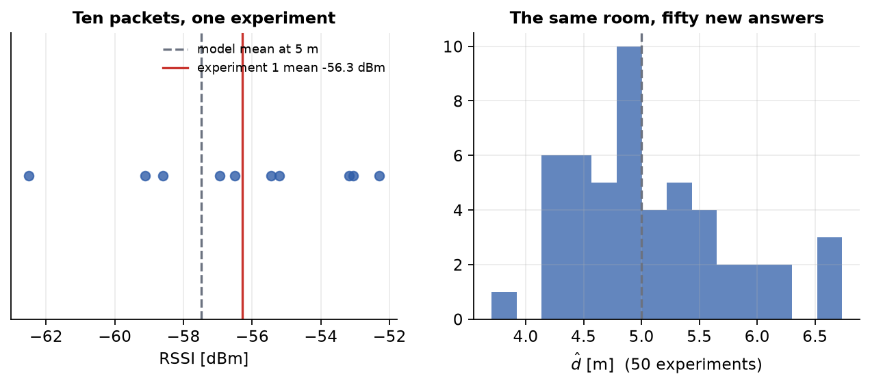
Concept check. Why does the cloud of fifty darts not centre exactly on 5 m, and why does it not matter for the question "is the estimator biased"? (Answer: fifty repetitions estimate the mean with error 0.678/\sqrt{50}\approx0.10 m; the closed-form bias is derived in section 7.)
2. Bias, variance and the exact MSE split
Idea. Add and subtract the estimator's own mean inside the square:
The cross term is 2(\mathbb E\hat\theta-\theta)\,\mathbb E[\hat\theta-\mathbb E\hat\theta]=0, because a centred variable has mean zero. What is left is an identity:
Risk under squared error is the same statement (wasserman2004_ea08 ↗, ch. 12; watkins2016_5a65, eq. 14.4).
Shrinkage. Estimate a receiver's mean RSSI excess \mu over a reference from N packets with per-packet noise \sigma=2 dB. Use \hat\mu_c=c\bar x. Its bias is (c-1)\mu and its variance is c^2\sigma^2/N, so
Setting the derivative to zero, -2(1-c)\mu^2+2c\sigma^2/N=0, gives
In words: total error is offset squared plus scatter; shrinking buys scatter with offset. The optimum needs \mu, the number being estimated. Unbiasedness is a guarantee across all \mu; shrinkage is a bet on \mu.
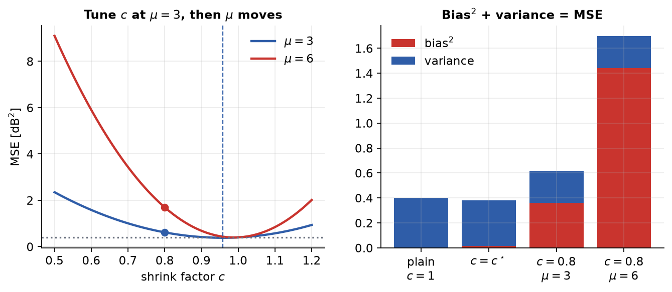
Worked numbers (widget default). \mu=3 dB, \sigma=2 dB, N=10 (closed form). Plain mean: bias^2=0, variance 0.400, MSE 0.400. Optimum: c^\star=0.9574, bias^2=0.0163, variance 0.3667, MSE 0.3830, a 4.3 % reduction. A 20,000-replicate Monte Carlo gives 0.3989 and 0.3815, a 4.4 % reduction. The widget's own 400 seeded darts give 0.410 and 0.390; they are illustrative and sit within sampling error of the closed form.
Break it. Set c=0.8 at \mu=3: MSE 0.616, already worse than the plain mean's 0.400, because the optimum at \mu=3 is c^\star=0.957, not 0.8. Now move the truth to \mu=6: MSE 1.696 (bias^2 1.440, variance 0.256) against 0.400 for the plain mean. The optimal c at \mu=6 is 0.989. Bias is immune to N, so a shrinkage tuned for the wrong \mu never recovers with more data.
Forward pointer. The rule for c^\star needs the unknown truth. Week 3 shows how a prior earns the shrinkage and replaces the forbidden confidence-interval reading with a credible set; Week 4 shows why shrinking across several receivers beats estimating each alone.
Concept check. Which term does averaging more data shrink, and which does it leave untouched? (Answer: variance falls as 1/N; bias is immune to N.)
3. Unbiased is a property, not a virtue: the divisor race
Idea. Estimate a variance from N Gaussian readings with SS=\sum(x_i-\bar x)^2. First the mean. Write each deviation from the sample mean through the deviation from the true mean \mu:
The cross terms collapse because \sum_i(x_i-\bar x)=0. Take expectations: the first sum gives N\sigma^2 and the second N\cdot\sigma^2/N=\sigma^2, so \mathbb E[SS]=(N-1)\sigma^2.
In words: the sample mean minimises the squared deviations of its own sample, so deviations measured from it fall short of deviations from the truth by exactly one observation's worth.
For Gaussian data SS/\sigma^2 is chi-square with N-1 degrees of freedom, so \mathrm{Var}(SS)=2(N-1)\sigma^4. For the divisor k, bias^2 plus variance gives
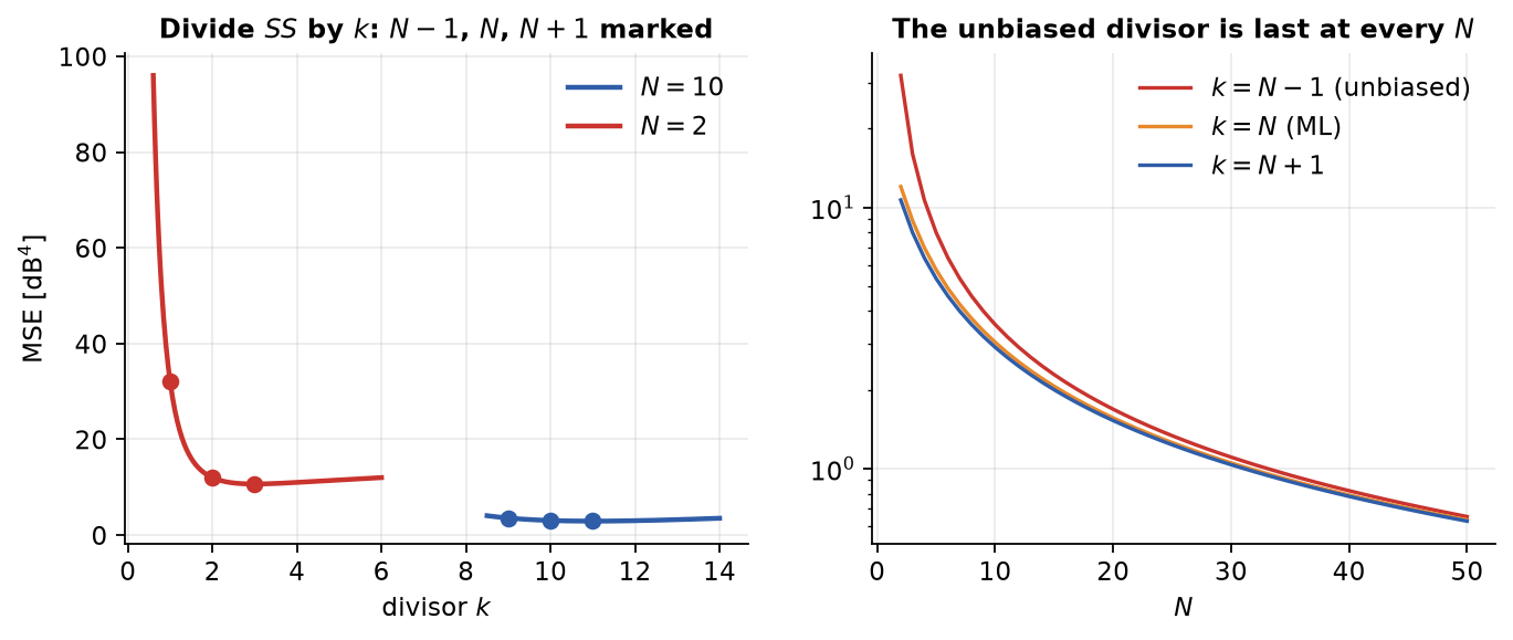
Minimising over k gives k=N+1. Three named divisors: k=N-1 is unbiased, k=N is the maximum-likelihood estimator, k=N+1 minimises MSE. In closed form \mathrm{MSE}(N-1)=2\sigma^4/(N-1), \mathrm{MSE}(N)=(2N-1)\sigma^4/N^2, \mathrm{MSE}(N+1)=2\sigma^4/(N+1), and the unbiased divisor is last of the three for every N from 2 to 200 (checked in the workbook). The corpus supports that the divide-by-N estimator beats the unbiased one in MSE in the normal family (gentle2020_1ba7, sections 5.1.4 and 5.1.5); that N+1 is the optimum is derived here, the corpus does not state it.
In words: dividing by a little more than you should adds a small shortfall and removes more scatter.
Worked numbers (widget default). N=10, \sigma^2=4 dB^2 (closed form): k=9, bias 0.000, MSE 3.556; k=10, bias -0.400, MSE 3.040; k=11, bias -0.727, MSE 2.909 (dB^4). The ratio of MSE at k=N to k=N-1 is 0.855. Monte Carlo (20,000 replicates): 3.565, 3.052, 2.924 and a mean SS of 35.94 against the theoretical 36.
Break it. Set N=2: unbiased MSE 32.0, k=N gives 12.0, k=N+1 gives 10.67. The gap grows as the sample shrinks.
Concept check. A sensor reports the sample variance of 3 readings. Which divisor would you choose to minimise the squared error of the variance, and which if the number feeds a later formula that needs its expectation to be right? (Answer: k=4 for MSE; k=2 when the expectation matters.)
4. Score and Fisher information: how loudly the data vote
Idea. The likelihood is the data density viewed as a function of the parameter, p(x;\theta). Its log is \ell(\theta). Differentiate with respect to the parameter to get the score,
The score has mean zero at the truth. Differentiate \int p(x;\theta)\,dx=1 under the integral:
In words: at the true parameter the data vote to move the estimate up exactly as often and as loudly as down.
Fisher information is the variance of the score, and one more derivative gives the curvature form:
Independent packets add log-likelihoods, hence scores, hence variances: I_N=N\,I_1. Information is a property of the measurement model; no estimator has been mentioned. A precision gain of one decimal digit costs a hundredfold more data.
Gaussian worked example. N packets with known \sigma: \ell(\mu)=-\sum(x_i-\mu)^2/(2\sigma^2)+\text{const}, s=n(\bar x-\mu)/\sigma^2, \partial^2_\mu\ell=-n/\sigma^2 (no randomness, so both forms agree), and
In words: a sharp peak pins the parameter; information is how sharp the peak is on average.
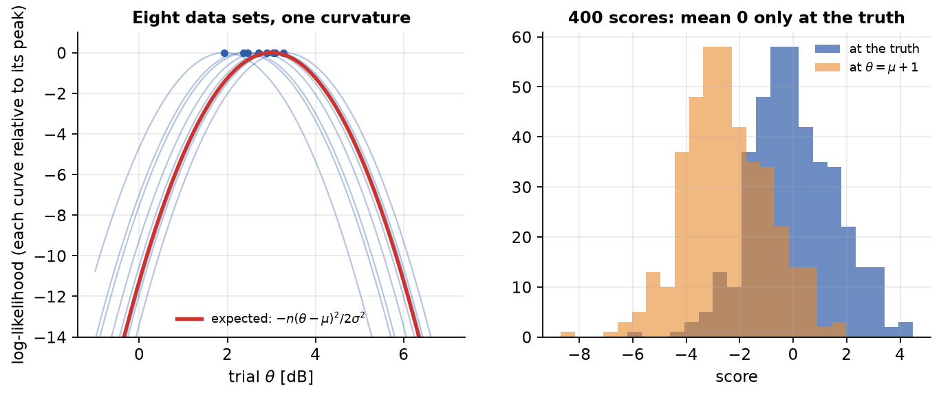
Worked numbers (widget default). \sigma=2 dB, n_{pkt}=10: I=2.50 per dB^2, floor sd 0.632 dB (closed form). The 400 seeded scores at the truth have mean 0.021 and variance 2.57 (theory 0 and 2.5). At a trial value 1 dB above the truth the mean score is -2.48 (theory -2.5): the score leaves zero when the trial value leaves the truth.
Break it. Set n_{pkt}=1 and \sigma=8 dB: I=0.0156 per dB^2, the likelihood curves are nearly flat, and the peaks of eight replicate data sets scatter with sd 8.1 dB (theory 8) across the whole axis.
Concept check (Poisson). For x\sim\mathrm{Poisson}(\lambda), \ln p=x\ln\lambda-\lambda-\ln x!, so s=x/\lambda-1 and I_1=\mathrm{Var}(x)/\lambda^2=1/\lambda. The floor for N counts is \lambda/N, and the sample mean sits on it. At \lambda=4, N=10 the floor is 0.400; a 20,000-replicate Monte Carlo of the sample-mean variance gives 0.396. This is the doorway to Week 2, which opens on counts.
5. The bound, and who reaches it
Proof. Let \hat\theta be unbiased for every \theta. Differentiate \int\hat\theta(x)\,p(x;\theta)\,dx=\theta under the integral. The estimator does not depend on \theta, so
Because \mathbb E[s]=0 this is \mathrm{Cov}(\hat\theta,s)=1. Every unbiased estimator has covariance exactly one with the score. Cauchy-Schwarz, \mathrm{Cov}^2\le\mathrm{Var}\,\mathrm{Var}, then gives
For an estimator with mean k(\theta) the same steps give \mathrm{Var}(\hat\theta)\ge k'(\theta)^2/I(\theta) (watkins2016_5a65, eqs. 14.10 to 14.17).
Efficiency. Rearranged, efficiency is a correlation:
Equality in Cauchy-Schwarz holds exactly when \hat\theta is a linear function of the score. At finite N an unbiased estimator on the bound exists only in a one-parameter exponential family, and the normal mean is one (gentle2020_1ba7, eq. 5.18 and Example 5.11). The maximum-likelihood estimator is asymptotically normal with variance 1/(nI), hence asymptotically efficient (watkins2016_5a65, asymptotic properties), and that optimality is predicated on the assumed model being correct (wasserman2004_ea08 ↗, section on optimality). Under a normal model the median has asymptotic relative efficiency 2/\pi=0.64 to the mean.
In words: every unbiased estimator is welded to the score with covariance one; the ones that follow it tightly reach the floor.
Regularity fine print. The proof interchanges derivative and integral twice. It needs the model to be smooth in \theta and the support of the data not to depend on \theta. Section 10 shows a model where that fails.
Worked numbers (widget default). 600 seeded replicates of N=11 packets, noise sd 2 dB, truth \theta=0. Gaussian noise: sample mean \rho^2=1.00 (it is linear in the score; the efficiency against the known I_N is 0.964, the difference is sampling error in the variance), median 0.654 (asymptotic reference 2/\pi=0.637), 20 % trimmed mean 0.901, first packet only 0.102. Laplace noise with the same sd (scale \sigma/\sqrt2, I_1=2/\sigma^2): sample mean \rho^2=0.535 (efficiency 0.504; exactly 0.5 at every N, because \mathrm{Var}(\bar x)=\sigma^2/N and 1/I_N=\sigma^2/(2N)), median 0.629 (efficiency 0.709, tending to 1.00), trimmed mean 0.683, first packet 0.051. At N=101 the Laplace efficiencies are 0.474 (mean) and 0.827 (median); the Gaussian median is 0.565.
The measured \mathrm{Cov}(\hat\theta,s) for the sample mean is 0.95, 1.01, 1.04 and 1.12 at N=3, 10, 11 and 101; the sampling error of a covariance from 600 replicates is about 0.06, so these are consistent with 1 (the last is at two standard errors). The efficiency of the Laplace rows rests on a textbook derivation that the corpus does not contain; the workbook shows it in closed form and by Monte Carlo. Older check: 20,000 replicates at N=50 give an efficiency ratio of 1.008, and 12 seeds give a mean 1.000 with a 2.5 to 97.5 percentile band of [0.985, 1.012].
Break it. Switch the noise to Laplace and keep the sample mean: the estimator that is best under a Gaussian model now wastes half the information, and the median wins. The Cramér-Rao bound is a property of the model, and so is "best".
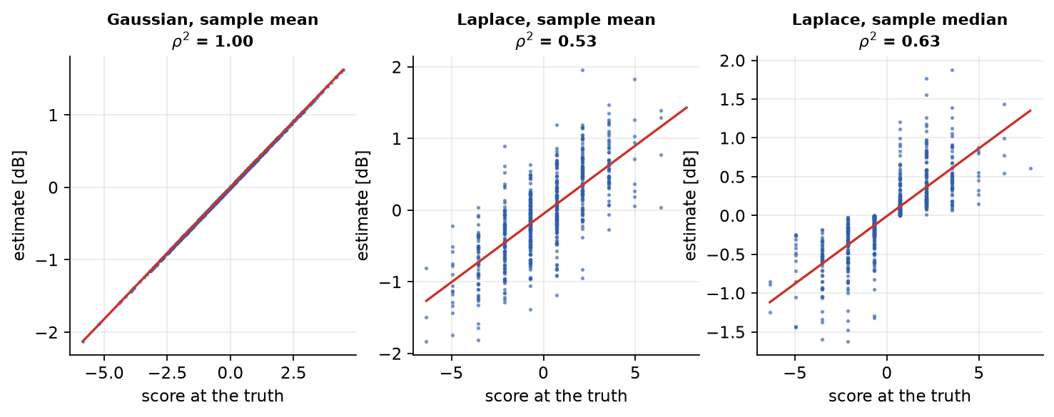
Concept check. Why can the first packet alone have covariance one with the score and still be a poor estimator? (Answer: covariance one is forced by unbiasedness; the correlation, hence the efficiency, also depends on how much variance the estimator adds beyond the score, and here it is \sigma^2 against \sigma^2/N.)
6. What the floor buys: a 95 % interval and its coverage
Idea. The square root of the floor is the standard error, \sigma/\sqrt N. The interval \bar x\pm z\,\sigma/\sqrt N, with z=1.960 for 95 %, is a procedure that traps the fixed \mu in 95 % of repetitions. The interval is random and the parameter fixed. The 95 % belongs to the recipe, not to the one interval on the screen; a probability statement about \theta given the data needs a prior (wasserman2004_ea08 ↗, section 6.3.2; the credible set is Week 3).
If the sample standard deviation s replaces \sigma and the same z is kept, the exact coverage is 2F_{t,N-1}(z)-1, where F_{t,N-1} is the Student t distribution function. It falls short of 95 % at small N because the t distribution has heavier tails. With the t quantile in place of z the coverage is nominal again.
Worked numbers (widget default). \mu=3 dB, \sigma=2 dB, N=10, 100 seeded intervals. Known \sigma with z: 94 of 100 cover; sample s with z: 93; sample s with t: 96. These are one seeded rain, not the procedure's coverage. Exact coverage of the procedure with known \sigma is 0.950 (a 20,000-repeat Monte Carlo gives 0.950). Exact coverage of s with z (closed form):
| N | 2 | 3 | 5 | 10 | 30 |
|---|---|---|---|---|---|
| coverage | 0.700 | 0.811 | 0.878 | 0.918 | 0.940 |
Break it. Toggle "sample s with z" and drop N to 3: exact coverage 0.811, and the seeded rain shows 78 of 100. Switch to t (t_{0.975,2}=4.303 against z=1.960) and the rain returns to 93 of 100 and the exact coverage to 0.950.
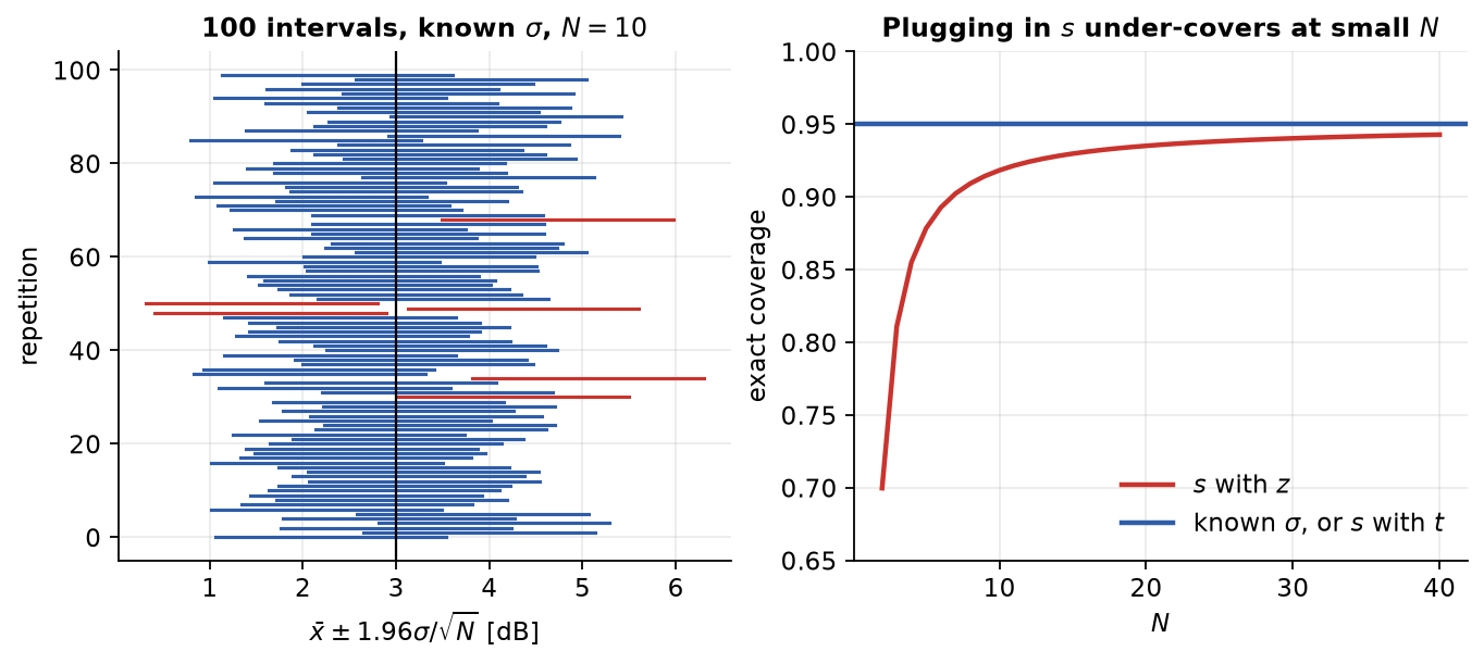
Concept check. A colleague writes "there is a 95 % probability that \mu lies in [3.1,4.3]". What does the 95 % refer to, and for which object would the sentence be correct? (Answer: the long-run capture rate of the procedure; the sentence is correct for a Bayesian credible interval given a prior.)
7. The ranging floor: RSSI under log-normal shadowing
Derivation in three moves.
- Average the packets. At fixed d, \bar P is Gaussian with mean \mu(d)=P_0-10n\log_{10}d and variance \sigma^2/n_{pkt}.
- Information about the mean. From section 4, \bar P carries I(\mu)=n_{pkt}/\sigma^2.
- Chain rule to distance. Only the mean depends on d, so I(d)=I(\mu)\,\mu'(d)^2 with \mu'(d)=-10n/(d\ln10):
Dimensional check: \sigma and 10n are both in dB per decade, so their ratio is dimensionless; times d gives metres.
In words: the achievable error is the distance, times shadowing over slope, over the square root of the packet count.
Three design consequences.
- Airtime buys the square root: four times the packets halve the floor (40 packets: 0.291 m). Inverting the bound gives the packet budget n_{pkt}=\big(d\sigma\ln10/(10n\,\mathrm{sd}_{target})\big)^2.
- The environment enters as \sigma/n: doubling \sigma to 8 dB doubles the floor to 1.165 m; doubling n to 5 halves it to 0.291 m.
- Relative error is constant in d: the floor is 1.165 m at d=10 m, still 11.65 % of d. RSSI ranging is a fixed-percentage instrument. The corpus notes that time-averaging is the common way to estimate mean RSS, and that the position error bound of RSS localisation grows with the shadowing variance, falls with the square of the path-loss exponent and depends on anchor angles (liu2022_9677 ↗, RSS-based localisation). The log-distance model with Gaussian shadowing is the standard model for RSSI ranging in Wi-Fi and BLE practice (roy2022_18d3 ↗; cantnpaterna2017_8af8 ↗), and multipath shadowing fundamentally limits RSSI-based ranging (fallani2026_04be ↗).
The estimator is log-normal. Substituting \bar P=\mu(d)+(\sigma/\sqrt{n_{pkt}})z into the inverse law gives \hat d=d\,e^{-sz} with s=\sigma\ln10/(10n\sqrt{n_{pkt}}) and z\sim\mathcal N(0,1). So \ln(\hat d/d)\sim\mathcal N(0,s^2): the exact mean is d\,e^{s^2/2} and the exact sd is d\sqrt{(e^{s^2}-1)e^{s^2}}. A convex transform biases upward, as the delta method says (watkins2016_5a65, eq. 14.8). The bound for an estimator whose mean is k(d)=d\,e^{s^2/2} is k'(d) times the unbiased floor, that is e^{s^2/2}\,d\,s. The bias-corrected estimator \hat d\,e^{-s^2/2} is unbiased with sd d\sqrt{e^{s^2}-1} and efficiency s^2/(e^{s^2}-1).
Worked numbers (widget default). d=5 m, \sigma=4 dB, n=2.5, n_{pkt}=10, so s=0.1165 (closed form):
| quantity | value |
|---|---|
| floor d\,s | 0.583 m (11.7 % of d) |
| ML estimator, exact sd | 0.588 m (ratio to floor 1.010) |
| ML estimator, exact bias | +0.034 m |
| bias-corrected sd, efficiency | 0.584 m, 0.993 |
| ML sd against the bound that applies to it | ratio 1.003 |
| packets for a floor of 0.4 / 0.2 / 0.1 m | 21.2 / 84.8 / 339.3 |
The floor of 0.583 m itself costs 10.0 packets. Monte Carlo cross-checks: 20,000 replicates give an ML sd of 0.589 m (ratio 1.011) and bias +0.028 m; the widget's 600 seeded draws give 0.586 m and +0.042 m.
Break it. Set n_{pkt}=1 at the defaults. The floor is 1.842 m, the exact ML sd is 2.040 m (ratio 1.108) and the bias is +0.351 m; the bias-corrected estimator has efficiency 0.934. Push \sigma to 10 dB and n to 1.6: floor 7.20 m, ML sd 37.1 m (ratio 5.15), bias +9.08 m. The bound describes an unbiased estimator near the truth; here the estimator is neither. The corpus records the general low-SNR failure of the Cramér-Rao bound and names Weiss-Weinstein and Ziv-Zakai (Bayesian) bounds as the tighter, costlier alternatives (liu2022_9677 ↗, estimation-theoretic metrics); it is silent on the low-packet-count regime of RSSI ranging specifically. The Bayesian bounds are a pointer here, not part of the week.
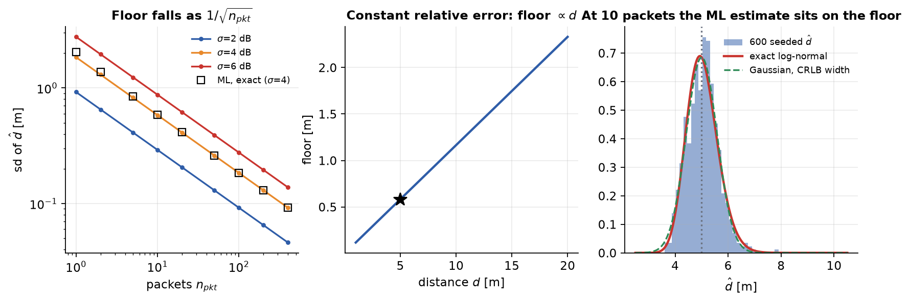
Concept check. A design needs 0.1 m at 5 m in the default environment. Give the packet count, then say what a 10 packets per second beacon means for the time per fix. (Answer: 339.3 packets, about 34 s.)
8. Several receivers: information becomes a matrix
Idea. With K receivers at known positions r_i and the transmitter at p, let d_i=\|p-r_i\| and u_i=(p-r_i)/d_i. Receiver i measures only distance, so its information about the position is rank one, along its own line of sight:
The position bound is F^{-1}; the RMS position floor is \sqrt{\mathrm{tr}\,F^{-1}}, and the one-sigma error ellipse has semi-axes equal to the square roots of the eigenvalues of F^{-1}. Geometry, not per-link noise, decides how well conditioned F is. The corpus says generically that RSS localisation bounds depend on the anchor angles (liu2022_9677 ↗); it is silent on any named dilution-of-precision quantity, so none is used here.
In words: each receiver only tells you how far along its own ray; you need rays from different directions.
Worked numbers (widget default). Four receivers at the corners of a 10 m square, transmitter at (3,4), \sigma=4 dB, n=2.5, n_{pkt}=10, so b=73.7. F=\begin{pmatrix}2.743&0.700\\0.700&3.842\end{pmatrix} per m^2, RMS floor 0.81 m, ellipse semi-axes 0.49 m and 0.65 m, condition number 1.74 (closed form). With two adjacent corners only the floor is 1.11 m.
Break it. Layout "three in a line", receivers at (0,0), (4,0), (10,0) (an assumption of the widget). With the transmitter exactly on the line F is singular: no receiver sees across it. Numerically, at 0.001 m off the line the condition number is 1.17\times10^{7}, the along-line sd is 0.20 m and the across-line sd is 684 m. That last number is a function of the 0.001 m offset, not a property of the layout: at 0.1 m off it is 6.85 m (condition number 1175) and at 1 m off it is 0.79 m (condition number 12.2).
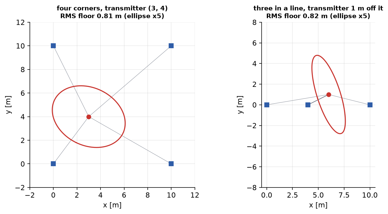
Concept check. Why does adding a fourth receiver next to the three on the line barely help, while one off the line helps at once? (Answer: information adds as matrices; only a ray with a component across the line adds information in that direction.)
9. Averaging cannot remove a bias: the measured hall
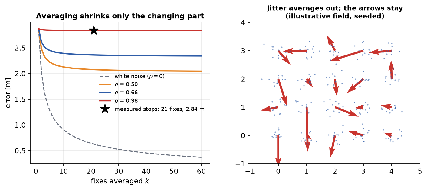
Idea. The square-root law of sections 4 to 7 assumes errors that are independent around the truth. Suppose a share \rho of each reading's error variance v is fixed to the place (multipath and hall geometry that the two-parameter model does not know) and the rest is independent per reading. Averaging k readings removes only the independent part:
As k\to\infty this tends to \sqrt{\rho v}, not to zero. In words: averaging shrinks the part of the error that changes between looks, not the part that belongs to the spot. A workbook simulation of exactly this model (20,000 cells, 21 looks) reproduces the formula: RMS after 21 looks 0.625 m at \rho=0, 2.077 m at \rho=0.5 and 2.862 m at \rho=0.98, against 0.626, 2.077 and 2.843 from the formula.
The measurement. A phone was carried through one large open university hall while advertising Bluetooth packets. Ten receivers ringed the hall and nine heard it. Every 2 s one position was solved independently from one log-distance model fitted to the same walk (fitted exponent 1.215, residual 2.86 dB). At 29 places the walker stood still, with a median of 21 fixes per stop. One fix at a stop missed by 2.87 m; the average of a stop missed by 2.84 m; independent errors would have given 2.87/\sqrt{21}=0.63 m. Averaging removed 1.2 % of the error where white noise would have removed 78.2 %. Over 2 m floor cells, 66.1 % of the error variance sat between cells, and the error autocorrelation was 0.68 over one 2 s bin and still 0.42 over seven. This is a single walk in a single hall, so it is one case of the failure, not an estimate of how common it is.
Worked numbers (widget default). k=21, v=2.87^2 m^2 (per-fix error 2.87 m), textbook \rho=0: predicted 0.63 m, measured 2.84 m. With \rho=0.5 the model gives 2.08 m and with \rho=0.661 (the between-cell share) 2.36 m, with a floor of 2.33 m as k grows. The share that reproduces the measured stop average is \rho\approx0.98. That value rests on an assumption: the source reports typical error magnitudes, and the calculation treats the ratio of those magnitudes as if it were an RMS ratio. The between-cell share (0.66) and the stop-based share (0.98) measure different things, and the two are not reconciled here.
What the bound would have promised. With the hall's own fitted parameters (\sigma=2.86 dB, n=1.215) the single-link floor at 5 m is 2.71 m for one reading and 0.59 m after 21 readings (closed form, a model computation with measured parameters, not a measurement). The bound was computed correctly and still describes nothing measured, because its model omits the fixed part. Maximum-likelihood optimality is predicated on the model being correct.
Break it. Slide \rho from 0 to 0.98 and watch the curve climb from the dashed white-noise line to the measured star. The corpus is silent on spatially correlated shadowing (decorrelation distance and related models), so the point here rests on the measurement above and on the variance-share argument.
Forward pointers. Week 5 turns this into dependence and the effective sample size; Week 10 into calibration and drift.
Concept check. A colleague proposes a Kalman filter on the position track to reach the 0.63 m. What part of the error can the filter act on? (Answer: only the part that changes between fixes; the fixed share stays.)
10. When the bound does not apply: a support that moves
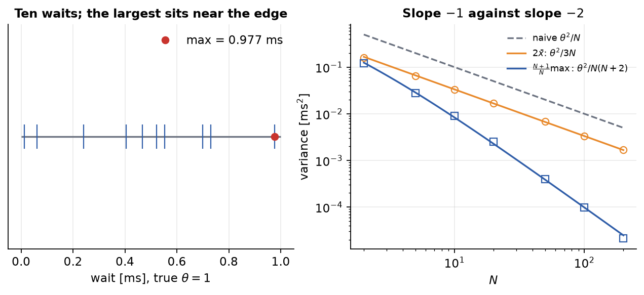
Counterexample. A device waits a uniform random time on [0,\theta] before replying; estimate \theta from N waits. One wait has density 1/\theta on [0,\theta], so \ln p=-\ln\theta and the naive score is -1/\theta with nonzero mean: the argument of section 4 already fails. Applying the formula regardless would give "information" 1/\theta^2 per wait and a floor \theta^2/N. Two estimators disagree with it:
- 2\bar x is unbiased with \mathrm{Var}=4\cdot\theta^2/(12N)=\theta^2/(3N), three times below the naive floor.
- \tfrac{N+1}{N}\max_i x_i is unbiased (\mathbb E[\max]=N\theta/(N+1)) with \mathrm{Var}=\tfrac{(N+1)^2}{N^2}\cdot\tfrac{N\theta^2}{(N+1)^2(N+2)}=\theta^2/(N(N+2)), falling as 1/N^2.
For the derivative-under-the-integral step to hold, the support must not depend on \theta; here it does, so the derivative acquires a boundary term (watkins2016_5a65, Exercise 14.19). The bound is a theorem with hypotheses, not a slogan.
In words: when the edge of the data moves with the parameter, one observation near the edge tells you a lot, and the Cramér-Rao argument does not apply.
Worked numbers (widget default). N=10, \theta=1 ms (closed form): naive floor 0.100 ms^2, 2\bar x 0.0333, \tfrac{N+1}{N}\max 0.00833. The widget's 2000-replicate Monte Carlo gives 0.0332 and 0.0090. The log-log slopes over N=2 to 200 are -0.99 and -1.88 from the Monte Carlo, against -1 and (asymptotically) -2 in closed form. The naive floor has slope -1.
Break it. This is the whole widget. The student is asked to find the step of the proof that fails: the interchange of derivative and integral.
Closing check, and the doorway to Week 2. Section 4's Poisson check ends the week's algebra with a count model: I_1=1/\lambda, the sample mean on the floor. Week 2 opens on counts, the number of packets or Bluetooth addresses a receiver hears per minute, and asks what the same machinery says when the variance is not equal to the mean.
Exam questions
Q1 (decomposition). Define bias, variance and MSE for \hat\theta of \theta, prove \mathrm{MSE}=\mathrm{bias}^2+\mathrm{Var}, and explain why the divide-by-N variance estimator can beat the unbiased divide-by-(N-1) estimator.
Model answer. Bias is \mathbb E\hat\theta-\theta, variance is \mathbb E[(\hat\theta-\mathbb E\hat\theta)^2], MSE is \mathbb E[(\hat\theta-\theta)^2]. Add and subtract \mathbb E\hat\theta, expand; the cross term contains \mathbb E[\hat\theta-\mathbb E\hat\theta]=0. For SS/k, \mathrm{MSE}=\sigma^4[(2(N-1)+(N-1)^2)/k^2-2(N-1)/k+1]. At N=10, \sigma^2=4 this is 3.556 for k=9 and 3.040 for k=10: the larger divisor adds a bias of -0.4 (bias^2 0.16) and removes more than that in variance.
Q2 (the bound). State the Cramér-Rao bound with its assumptions and prove it. Give a model where the assumptions fail and say what goes wrong.
Model answer. For an estimator unbiased for every \theta, in a model smooth in \theta with support independent of \theta, \mathrm{Var}(\hat\theta)\ge1/I(\theta). Proof: differentiate \mathbb E\hat\theta=\theta to get \mathrm{Cov}(\hat\theta,s)=1, then Cauchy-Schwarz. Counterexample: uniform on [0,\theta]. The score has mean -1/\theta\neq0, the naive floor is \theta^2/N, and \tfrac{N+1}{N}\max has variance \theta^2/(N(N+2)), which is below it for every N\ge1 (N(N+2)>N^2).
Q3 (worked bound). For the RSSI model derive the floor for \hat d. With d=5 m, \sigma=4 dB, n=2.5, n_{pkt}=10 evaluate it, and find the packets for a 0.2 m floor.
Model answer. I(d)=n_{pkt}(10n/(d\sigma\ln10))^2; floor =d\sigma\ln10/(10n\sqrt{n_{pkt}})=5\cdot4\cdot2.303/(25\cdot3.162)=0.583 m. For 0.2 m: n_{pkt}=10\,(0.5825/0.2)^2=84.8 packets, four times the packets for half the error after 21.2 for 0.4 m.
Q4 (interpretation trap). A colleague computes \bar x\pm1.96\,\sigma/\sqrt N=[3.1,4.3] and writes "there is a 95 % probability that \mu lies between 3.1 and 4.3". Is the sentence correct?
Model answer. No. The 95 % is the long-run capture rate of the procedure over repetitions with \mu fixed; after the data are seen the interval either contains \mu or does not. The sentence is correct for a credible interval under a prior. If s replaced \sigma with z kept, the actual capture rate at N=3 would be 0.811.
Q5 (geometry). Four receivers ring a room, and a fifth is added beside the fourth. Then all are moved onto one wall. Using the information matrix, say what changes for the position floor and why, without any new noise per link.
Model answer. F=\sum_i(b/d_i^2)u_iu_i^T. A receiver beside another adds a nearly parallel rank-one term, so the eigenvalue in the other direction barely moves. On one wall with the transmitter on that wall's line, all u_i are parallel, F is singular and the across-line variance is unbounded; at 0.001 m off the line the across-line sd is 684 m for the workbook layout, while the along-line sd stays 0.20 m. Geometry, not per-link noise, sets the conditioning.
Q6 (averaging). A stationary transmitter is located 21 times in a row; each fix is off by about 2.9 m and the mean of the 21 is off by 2.8 m. What does this say about the error, and does the Cramér-Rao floor for the single-link model (0.59 m after 21 readings) contradict the measurement?
Model answer. Independent errors would leave 2.9/\sqrt{21}=0.63 m; almost nothing averaged out, so the error is nearly all fixed to the place (\rho near 1 under the RMS assumption). The floor does not contradict the measurement: it is correct for its model, and the model omits the fixed part. Optimality of the maximum-likelihood estimator is predicated on the model being correct.
Further reading
- wasserman2004_ea08 ↗: risk, confidence-set semantics, MLE efficiency and the model-correctness caveat, median efficiency 2/\pi.
- gentle2020_1ba7: the information inequality, attainment only in the one-parameter exponential family, divide-by-N against the unbiased variance estimator.
- watkins2016_5a65: score, Fisher information, the Cauchy-Schwarz proof in the k'(\theta)^2/I form, the uniform exercise, delta-method bias, MLE asymptotics.
- liu2022_9677 ↗: scaling of RSS localisation bounds, the low-SNR failure of the Cramér-Rao bound and the Bayesian bounds.
- stoica1989_614d ↗: estimators approaching the bound in array processing, for further reading only.
- roy2022_18d3 ↗, cantnpaterna2017_8af8 ↗ and fallani2026_04be ↗: the log-distance model in practice and the limit that multipath shadowing sets.
The corpus is silent on: Kay's Fundamentals of Statistical Signal Processing (not in the vault), the original Cramér-Rao papers and their history, spatially correlated shadowing, and the low-packet-count behaviour of RSSI ranging estimators. Nothing on those is cited here.
Provenance (instructor only)
Not for the deck or for students. Vault paths of the sources behind first-party numbers and corpus claims:
obsidian/monad-knowledge/diary/2026-09-09 - Filtering the BLE track removes the bounce and cannot remove the miss, because two thirds of the miss is a bias fixed to the room.md(section 9: ten receivers, nine heard, exponent 1.215, residual 2.86 dB, 29 stops, median 21 fixes, 2.87 m, 2.84 m, 0.63 m, 1.2 %, 78.2 %, 66.1 %, autocorrelation 0.68 and 0.42)obsidian/monad-knowledge/edu/courses/PRB504-probabilistic-statistical-methods/week-01-estimation-theory-the-crlb/workbook.ipynbandnumbers.json(every other scalar)obsidian/monad-knowledge/literature/All of Statistics.mdobsidian/monad-knowledge/literature/Theory of Statistics.mdobsidian/monad-knowledge/literature/An Introduction to the Science of Statistics From Theory to Implementation.mdobsidian/monad-knowledge/literature/A Survey on Fundamental Limits of Integrated Sensing and Communication.mdobsidian/monad-knowledge/literature/MUSIC, maximum likelihood, and Cramer-Rao bound.mdobsidian/monad-knowledge/literature/A survey on ubiquitous WiFi-based indoor localization system for smartphone users from implementation perspectives.mdobsidian/monad-knowledge/literature/A Bluetooth Low Energy Indoor Positioning System with Channel Diversity, Weighted Trilateration and Kalman Filtering.mdobsidian/monad-knowledge/literature/IoT solutions for e-Health applications for care's continuity at home.md